Is there some problem in my understanding that this inequality is convex?
% Clear workspace and any previous CVX blocks
clear all;
cvx_clear;
% Start timing the process
tic;
% Define problem parameters
n = 12; % Number of state-action pairs (3 states * 4 actions)
K = 2; % Number of constraints (now simplified to 2)
Mc = 2; % Number of components in the mixture for the cost function (simplified)
Mdk = [2, 2]; % Two components for each of the 2 constraints
eta = 0.99; % Discount factor
% Transition probability matrices for each action A = 0, 1, 2, 3
P = cell(4, 1);
P{1} = [1, 0, 0; 0.67, 0.33, 0; 0.33, 0.33, 0.34];
P{2} = [0.67, 0.33, 0; 0.33, 0.34, 0.33; 0, 0.33, 0.67];
P{3} = [0.34, 0.33, 0.33; 0, 0.33, 0.67; 0, 0, 1];
P{4} = [0.34, 0.33, 0.33; 0, 0.33, 0.67; 0, 0, 1];
% Define Sigma, mu, xi, and weights for the upper bound
Sigma_ci = rand(n,n,Mc); % Covariance matrices for upper bound components
mu_ci = rand(n,Mc); % Mean vectors for upper bound components
Sigma_dk = rand(n,n,max(Mdk)); % Covariance matrices for demand constraints
mu_dk = rand(n,max(Mdk)); % Mean vectors for demand constraints
% Define xi_k (bounds) for each constraint k
xi_k = rand(K,1); % Bound on each constraint
% Prespecified weights normalized to sum to 1
p0 = 0.95; % Example values for p0 and p1
p1 = 0.95;
% Define prespecified weights satisfying conditions for upper bound and constraints
wi = [2*(1-p0); 2*(1-p0)]; % Two components for the upper bound
wk_j = {
[2*(1-p1), 2*(1-p1)], % Weights for the first constraint
[2*(1-p1), 2*(1-p1)] % Weights for the second constraint
};
% Normalize weights
wi = wi / sum(wi);
for k = 1:K
wk_j{k} = wk_j{k} / sum(wk_j{k});
end
% Number of interpolation points
N = 5; % Number of interpolation points for eta and delta
% Define interpolation points for eta and delta, ensuring the first point is slightly greater than 0
small_value = 1e-5; % Small value to avoid -infinity issue with norminv(0)
eta_interp = linspace(small_value, 1, N); % Interpolation points for eta_i^l
delta_interp = linspace(small_value, 1, N); % Interpolation points for delta_j^k
% Compute the absolute value of the inverse CDF for eta and delta (using norminv for normal distribution)
Phi_inv_eta = abs(norminv(eta_interp)); % |Inverse CDF| for eta interpolation
Phi_inv_delta = abs(norminv(delta_interp)); % |Inverse CDF| for delta interpolation
% Initialize arrays for a_i^l, b_i^l for the upper bound (Mc components)
ai = zeros(Mc, N-1); % a_i^l for each i and l
bi = zeros(Mc, N-1); % b_i^l for each i and l
% Initialize arrays for a_{j,l}^k, b_{j,l}^k for the constraints (K constraints)
ajk = cell(K, 1);
bjk = cell(K, 1);
for k = 1:K
ajk{k} = zeros(Mdk(k), N-1); % a_{j,l}^k for each j, l, k
bjk{k} = zeros(Mdk(k), N-1); % b_{j,l}^k for each j, l, k
end
% Compute a_i^l and b_i^l for the upper bound
for i = 1:Mc
for l = 1:(N-1)
ai(i, l) = (Phi_inv_eta(l) * eta_interp(l+1) - Phi_inv_eta(l+1) * eta_interp(l)) / max(eta_interp(l+1) - eta_interp(l), 1e-6);
bi(i, l) = (Phi_inv_eta(l+1) - Phi_inv_eta(l)) / max(eta_interp(l+1) - eta_interp(l) , 1e-6);
end
end
% Compute a_{j,l}^k and b_{j,l}^k for the constraints
for k = 1:K
for j = 1:Mdk(k)
for l = 1:(N-1)
ajk{k}(j, l) = (Phi_inv_delta(l) * delta_interp(l+1) - Phi_inv_delta(l+1) * delta_interp(l)) / max(delta_interp(l+1) - delta_interp(l) , 1e-6);
bjk{k}(j, l) = (Phi_inv_delta(l+1) - Phi_inv_delta(l)) / max(delta_interp(l+1) - delta_interp(l) , 1e-6);
end
end
end
% Initial distribution over states (gamma) for Qb(gamma)
gamma = ones(3, 1) / 3; % Uniform distribution for 3 states
% -----------------------------------------
% Step 1: Solve for V_i and V_{jk} by maximizing the sum with the Q_b(gamma) constraints
% -----------------------------------------
% Initialize Vi and Vjk
Vi = zeros(Mc, 1); % To store the V_i terms
Vjk = cell(K, 1); % To store the V_{jk} terms for each constraint
for k = 1:K
Vjk{k} = zeros(Mdk(k), 1);
end
% Solve for each Vi
for i = 1:Mc
cvx_begin
variable rho_i(n) % Decision variable rho for this specific optimization
maximize( sum( rho_i’ * vecnorm(Sigma_ci(:,:,i).^0.5, 2, 2) ) )
    % Constraints that rho_i belongs to Q_b(gamma)
    for s_prime = 1:3
        lhs_sum = 0;
        for s = 1:3
            for a = 1:4
                lhs_sum = lhs_sum + rho_i((s-1)*4 + a) * (kronecker_delta(s_prime, s) - eta * P{a}(s_prime, s));
            end
        end
        lhs_sum == (1 - eta) * gamma(s_prime);
    end
    sum(rho_i) == 1;
    rho_i >= 0;  % Non-negativity constraint on rho
cvx_end

% Store the optimal value of Vi
Vi(i) = cvx_optval;  % Store the optimal value of this subproblem
end
% Solve for each Vjk
for k = 1:K
for j = 1:Mdk(k)
cvx_begin
variable rho_jk(n) % Decision variable rho for this specific optimization
maximize( sum( rho_jk’ * vecnorm(Sigma_dk(:,:,j).^0.5, 2, 2) ) )
        % Constraints that rho_jk belongs to Q_b(gamma)
        for s_prime = 1:3
            lhs_sum = 0;
            for s = 1:3
                for a = 1:4
                    lhs_sum = lhs_sum + rho_jk((s-1)*4 + a) * (kronecker_delta(s_prime, s) - eta * P{a}(s_prime, s));
                end
            end
            lhs_sum == (1 - eta) * gamma(s_prime);
        end
        sum(rho_jk) == 1;
        rho_jk >= 0;  % Non-negativity constraint on rho
    cvx_end

    % Store the optimal value of Vjk
    Vjk{k}(j) = cvx_optval;  % Store the optimal value of this subproblem
end
end
% -----------------------------------------
% Step 2: Proceed with the main CVX optimization problem
% -----------------------------------------
cvx_begin
variable rho(n) % decision variable (probabilities over state-action pairs)
variable t % objective value
% Declare variables
variables yk(K) eta_var(Mc) delta_kj_var(K, max(Mdk)) zi(Mc) zkj(K, max(Mdk))
% Auxiliary variables for reformulating the product terms
variables aux_bi_eta(Mc, N-1) nonnegative % Auxiliary variable for bi(i, l) * eta_var(i)
% Apply nonnegativity constraints
yk >= 0;
eta_var >= 0;
eta_var <= 1;
delta_kj_var >= 0;
delta_kj_var <= 1;
zi >= 0;
zkj >= 0;
% Reformulated Qb(gamma) constraints (sum of probabilities must equal 1 and match transitions)
for s_prime = 1:3
sum_s_prime = sum(sum(rho((s_prime-1)*4 + (1:4)))); % Sum of probabilities for state s_prime
constraint_rhs = (1 - eta) * gamma(s_prime);
lhs_sum = 0;
for s = 1:3
for a = 1:4
% Use kronecker_delta function instead of delta
lhs_sum = lhs_sum + rho((s-1)*4 + a) * (kronecker_delta(s_prime, s) - eta * P{a}(s_prime, s));
end
end
lhs_sum == constraint_rhs; % Linear constraint using transition probabilities and delta function
end
% Ensure sum of probabilities is 1
sum(rho) == 1;
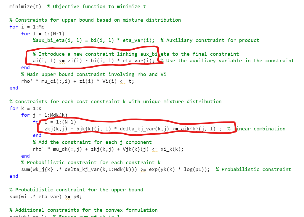
minimize(t) % Objective function to minimize t
% Constraints for upper bound based on mixture distribution
for i = 1:Mc
for l = 1:(N-1)
%aux_bi_eta(i, l) = bi(i, l) * eta_var(i); % Auxiliary constraint for product
% Introduce a new constraint linking aux_bi_eta to the final constraint
ai(i, l) <= zi(i) - bi(i, l) * eta_var(i); % Use the auxiliary variable in the constraint
end
% Main upper bound constraint involving rho and Vi
rho' * mu_ci(:,i) + zi(i) * Vi(i) <= t;
end
% Constraints for each cost constraint k with unique mixture distribution
for k = 1:K
for j = 1:Mdk(k)
for l = 1:(N-1)
zkj(k,j) - bjk{k}(j, l) * delta_kj_var(k,j) >= ajk{k}(j, l) ; % Linear combination
end
% Add the constraint for each j component
rho' * mu_dk(:,j) + zkj(k,j) + Vjk{k}(j) <= xi_k(k);
end
% Probabilistic constraint for each constraint k
sum(wk_j{k} .* delta_kj_var(k,1:Mdk(k))) >= exp(yk(k) * log(p1)); % Probabilistic constraint
end
% Probabilistic constraint for the upper bound
sum(wi .* eta_var) >= p0;
% Additional constraints for the convex formulation
sum(yk) == 1; % Ensure sum of yk is 1
cvx_end
% End timing
elapsedTime = toc; % Record the time taken
% Save the inputs, outputs, and the time
save(‘simplified_experiment_results.mat’, ‘n’, ‘K’, ‘Mc’, ‘Mdk’, ‘Sigma_ci’, ‘mu_ci’, ‘Sigma_dk’, ‘mu_dk’, ‘wk_j’, …
‘xi_k’, ‘p0’, ‘p1’, ‘rho’, ‘t’, ‘yk’, ‘eta_var’, ‘delta_kj_var’, ‘zi’, ‘zkj’, ‘elapsedTime’, ‘ai’, ‘bi’, ‘ajk’, ‘bjk’, ‘Vi’, ‘Vjk’);
% Display the computational time
fprintf(‘Optimization completed in %.4f seconds\n’, elapsedTime);
% Define Kronecker delta function
function result = kronecker_delta(s_prime, s)
if s_prime == s
result = 1;
else
result = 0;
end
end