There is actually one entry 0.0072 which is very small ,I believe it could be negligible.
I have another question
Is there a way where I could modify the constraints in such a way that I could get a sparser matrix? Please let me know.
There is actually one entry 0.0072 which is very small ,I believe it could be negligible.
I have another question
Is there a way where I could modify the constraints in such a way that I could get a sparser matrix? Please let me know.
You could try doing something with a vector one norm in the objective or a constraint, which perhaps might help induce sparsity. But how to induce sparsity is a modeling question outside the scope of this forum.
Hi again. I am a bit confused in giving a positive semidefinite constraint in cvx for my Euclidean Projection problem. I have two versions of my function
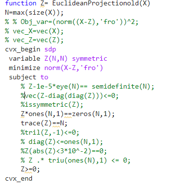
where I used sdp solver and then I added Z>=0 as a constraint in order to obtain the positive semidefinite matrix.
The other version is
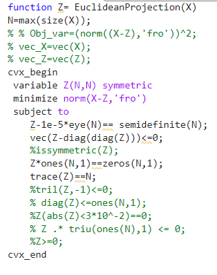
where I dont use sdp and Z>=0 constraint instead I use semidefinite(n).
What is the difference between both these versions. I have two sets of data. One from the power and the other is weather. The first version works perfectly well for power but fails in weather data but the second version works perfectly well for weather but fails in power.
You would need Z - 1e-5*eye(N) >= 0 in the first version for the semidefinite constraint to be the same as the 2nd version. The first version is missing vec(Z-diag(diag(X))) <= 0, which is in the 2nd version.
A follow-up of my comment in this link above.
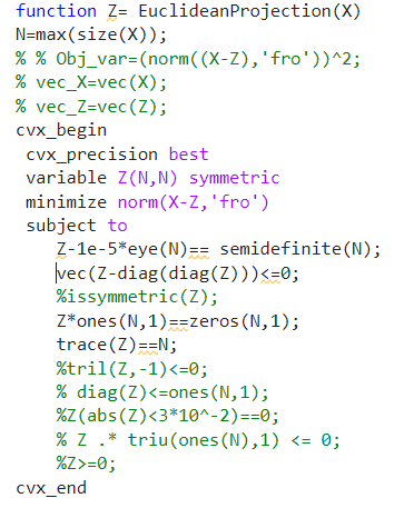
This version of Euclidean Projection perfectly well.
But this time I had to normalize/divide my input signal with a small coefficient (like a scalar value=0.005).
When I run this function on those signals cvx status is shown as Failed with optval as NaN but then the final result which I got is a valid Laplacian matrix satisfying all of the constraints. The graph I procured from this Laplacian matrix is also perfectly good after visualizing it.
If I comment the constraint vec(Z-diag(diag(X))) <= 0 and run my cvx code. The status now is solved with some optvalue but the final result is not a valid Laplacian since it fails to meet vec(Z-diag(diag(X))) <= 0 constraint.
This looks a bit confusing for me.
Hello Dr Stone
Another help.
A quick recall of my Euclidean Projection code.
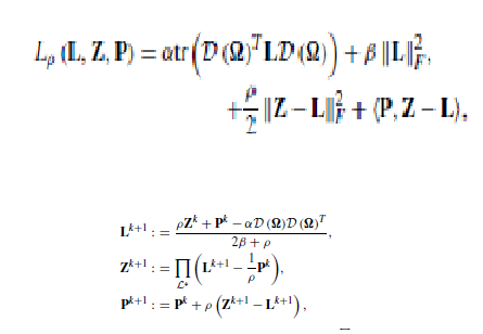
This is an ADMM implementation which uses Euclidean Projection. D(\omega) is the input signal.
The alpha,beta, and rho are the key parameters for regularizing the entries in the Laplacian.
vec(Z-diag(diag(Z)))<=0 is the constraint used to get positive edge weights of my final graph Laplacian.
trace(L)==N is the constraint used for normalizing the graph Laplacian
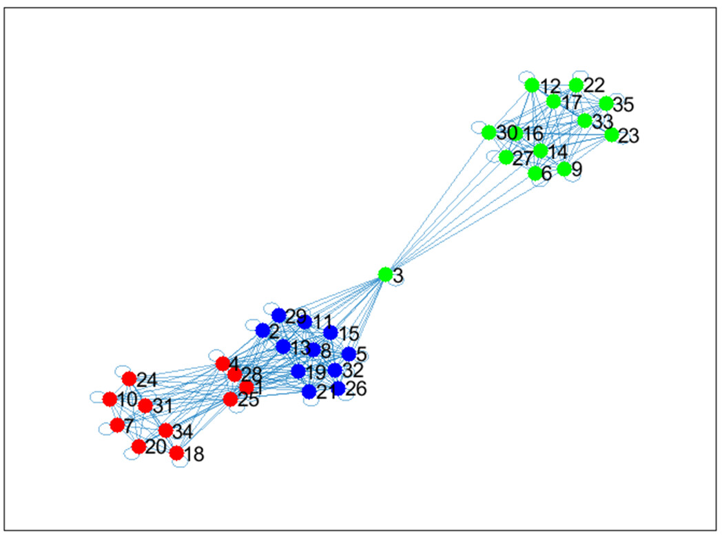
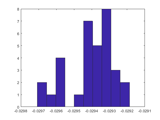
The distribution of the edge weights/entries of the learnt Laplacian is
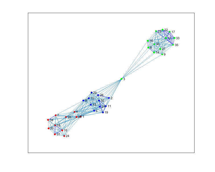
The graph visualization on this optimized matrix is
And here the weights are almost equal. There is a very small variation on entries. The graph initially is not sparse. I have thresholded some of the values to get that graph partition.
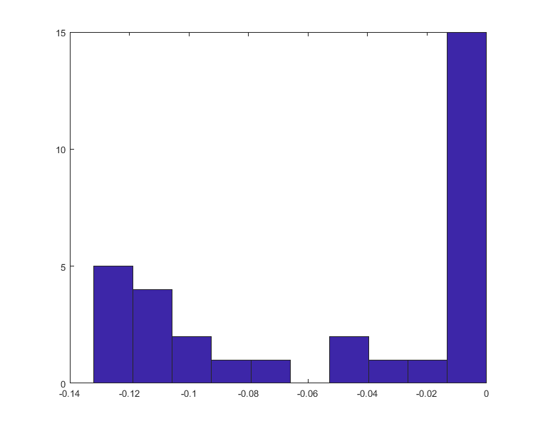
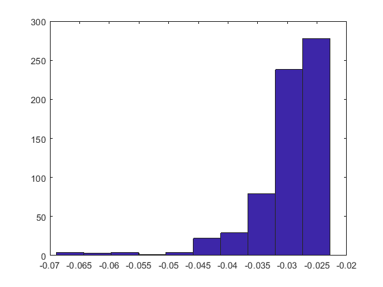
I am comparing this with a similarity graph where the Laplacian matrix(normalized) is based on the exponential on the Euclidean Distances in the signals.
Here is the histogram of the Laplacian entries and there are is bigger variation of these entries. The zeros are obtained after thresholding some of the values.
The graph visualization is given below.
The graph visualization is good in both the cases. However I dont see a good variation of the entries in the optimized Laplacian and I am skeptical about them. I have tried with many values of alpha,beta and rho starting from smaller values such as 0.1, 0.2 to larger values like 100 etc. cvx fails(giving infeasible solution) at very large values of these parameters.
I suspect that it has something to do with vec(Z-diag(diag(Z)))<=0.
Is there a way to tweak this constraint so that I could get the desired distribution of the entries (but not at the cost of graph partition).
I will be switiching to SeDuMi to try this in that solver.
I don’t have the application subject matter expertise to make a meaningful suggestion. Given the topic of this forum, it is not reasonable to expect readers to have such expertise. Nevertheless, if anyone wants to weigh in, they are welcome to do so.
Just changed to SeDuMi. No significant change in the constraints nor in the alpha,beta, and rho parameters.
Here is the histogram of the entries
but my graph is not promising.
Can you please let me know the difference in what SeDuMi does over SDPT3 on the same cost function and the constraints?
They are different solvers. They might not produce “exactly” the same solution even if it is unique. If there are non-unique solutions (i.e., multiple global optima), different solvers might end up at different solutions. Even changing the order of constraints provided to the solver, and maybe in user’s CVX program, could change which solution is obtained by a given solver. I
If there is some change to the objective or constraints which forces or encourages the solver to find a solution you “like”, you will have to figure that out. Or solve several problems and choose the solution you like.