The optimization variables in the formula has been multiplied by 0, why their optimization results are not 0 or infinitesimal

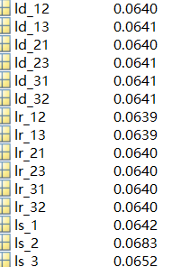
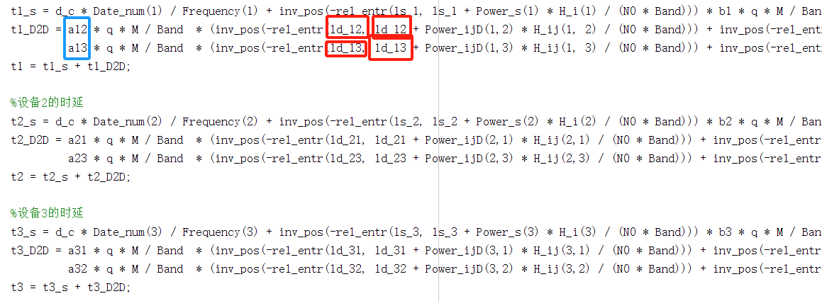
Hello everyone, thank you in advance for your help. I use cvx to optimize several variables. In the objective function, the formula in which some optimization variables are located is multiplied by 0, but their optimization results are not 0, or even large. May I ask why this situation occurs? And cvx often fails to solve, but I checked that my objective function and constraints are convex, hoping to help me find the problem, thank you very much.Here’s my code.

% Include CVX and set the solver to Mosek
% addpath('/path/to/cvx');
% cvx_setup;
% clear all;
cvx_solver mosek;

% Clear CVX environment
cvx_clear;

% Define problem data

C = 64; % Quantization bits
q = 64;
V = 0.5; % Lyapunov weight
alpha = 1;
Round_num = 1000; % Total rounds of training
Device_num = 3; % Number of devices
Date_num = 128 * ones(1, Device_num); % Data amount for each device
d_c = 0.1; % Compute resource requirement
M = 878538;

% Power definitions
% Generate a vector of random numbers following a normal distribution
mu = 0;
sigma = 1;
rand_nums = mu + sigma * randn(1, Device_num);

% Standardize the random number vector
rand_nums = (rand_nums - mean(rand_nums)) / max(abs(rand_nums)) * 1;

% Compute Power_s
Power_s = 1.0 * ones(1, Device_num) - 0.05 * rand_nums;

% Compute Power_ijD
Power_ijD = 1.0 * ones(Device_num, Device_num) - 0.05 * rand_nums;

% Compute Power_jir
Power_jir = 1.0 * ones(Device_num, Device_num) - 0.05 * rand_nums;

a = zeros(Device_num);
b = ones(1, Device_num);
%b(1) = 0;
%a(1,2) = 1;
Frequency = 1.5 * ones(1, Device_num) - 0.1 * rand_nums;
Band = 2e7;
Min_bandwidth = 0.1 / Device_num;
N0 = dBm_to_P(-174) * Band;

% Compute channel gain from users to the base station
H_i = zeros(1, Device_num);
d = 1; % Distance in kilometers

% Randomly distribute devices
base_station = [0, 0];

% Generate random user coordinates
Device_num = 3;
theta = 2 * pi * rand(1, Device_num);
radius = 200 * rand(1, Device_num);

% Convert polar coordinates to Cartesian coordinates
users_x = base_station(1) + radius .* cos(theta);
users_y = base_station(2) + radius .* sin(theta);
users_coordinates = [users_x; users_y];

% Calculate the distance from each device to the base station
Distance_i = sqrt((users_coordinates(1, :) - base_station(1)).^2 + ...
                            (users_coordinates(2, :) - base_station(2)).^2);

% Calculate the distance between devices
Distance_ij = zeros(Device_num, Device_num);
for i = 1:Device_num
    for j = 1:Device_num
        Distance_ij(i, j) = sqrt((users_coordinates(1, i) - users_coordinates(1, j)).^2 + ...
                                        (users_coordinates(2, i) - users_coordinates(2, j)).^2);
    end
end


% Compute channel gain from users to the base station
for k = 1:Device_num
    H_i(k) = channel_gain(Distance_i(k));
end

% Compute channel gain between users
H_ij = zeros(Device_num, Device_num);
for i = 1:Device_num
    for j = 1:Device_num
        H_ij(i, j) = channel_gain(Distance_ij(i, j));
    end
end

T_total = [];
D2D_total = [];
E_final = [];
D2D_energy_total = [];
t_D2D = 0;
Energy_coefficient = 0.1; % Energy efficiency
n_iterations = 20;
a12 = 0;
a21 = 0;
a13 = 0;
a31 = 0;
a23 = 0;
a32 = 0;
b1 = 1;
b2 = 1;
b3 = 1;
% for iteration = 1:n_iterations
    % Define CVX variables
    cvx_begin
        variable ls_1
        variable ls_2
        variable ls_3
        variable ld_12
        variable ld_21
        variable ld_13
        variable ld_31
        variable ld_23
        variable ld_32
        variable lr_12
        variable lr_21
        variable lr_13
        variable lr_31
        variable lr_23
        variable lr_32 
        variable T
        
        expression t1_s
        expression t1_D2D
        expression t1
        expression t2_s
        expression t2_D2D
        expression t2
        expression t3_s
        expression t3
        
        % Three devices
        % Device 1 delay
        % Direct upload to the base station delay
        t1_s = d_c * Date_num(1) / Frequency(1) + inv_pos(-rel_entr(ls_1, ls_1 + Power_s(1) * H_i(1) / (N0 * Band))) * b1 * q * M / Band;
        t1_D2D = a12 * q * M / Band  * (inv_pos(-rel_entr(ld_12, ld_12 + Power_ijD(1,2) * H_ij(1, 2) / (N0 * Band))) + inv_pos(-rel_entr(lr_21, lr_21 + Power_jir(2, 1) * H_i(2) / (N0 * Band)))) + ...
                 a13 * q * M / Band  * (inv_pos(-rel_entr(ld_13, ld_13 + Power_ijD(1,3) * H_ij(1, 3) / (N0 * Band))) + inv_pos(-rel_entr(lr_31, lr_31 + Power_jir(3, 1) * H_i(3) / (N0 * Band))));
        t1 = t1_s + t1_D2D;

        % Device 2 delay
        t2_s = d_c * Date_num(2) / Frequency(2) + inv_pos(-rel_entr(ls_2, ls_2 + Power_s(2) * H_i(2) / (N0 * Band))) * b2 * q * M / Band;
        t2_D2D = a21 * q * M / Band  * (inv_pos(-rel_entr(ld_21, ld_21 + Power_ijD(2,1) * H_ij(2,1) / (N0 * Band))) + inv_pos(-rel_entr(lr_12, lr_12 + Power_jir(1,2) * H_i(1) / (N0 * Band)))) + ...
                 a23 * q * M / Band  * (inv_pos(-rel_entr(ld_23, ld_23 + Power_ijD(2,3) * H_ij(2,3) / (N0 * Band))) + inv_pos(-rel_entr(lr_32, lr_32 + Power_jir(3, 2) * H_i(3) / (N0 * Band))));
        t2 = t2_s + t2_D2D;

        % Device 3 delay
        t3_s = d_c * Date_num(3) / Frequency(3) + inv_pos(-rel_entr(ls_3, ls_3 + Power_s(3) * H_i(3) / (N0 * Band))) * b3 * q * M / Band;
        t3_D2D = a31 * q * M / Band  * (inv_pos(-rel_entr(ld_31, ld_31 + Power_ijD(3,1) * H_ij(3,1) / (N0 * Band))) + inv_pos(-rel_entr(lr_13, lr_13 + Power_jir(1,3) * H_i(1) / (N0 * Band)))) + ...
                 a32 * q * M / Band  * (inv_pos(-rel_entr(ld_32, ld_32 + Power_ijD(3,2) * H_ij(3,2) / (N0 * Band))) + inv_pos(-rel_entr(lr_23, lr_23 + Power_jir(2, 3) * H_i(2) / (N0 * Band))));
        t3 = t3_s + t3_D2D;


        minimize(T);

        % Add constraints
        subject to
              ls_1 >= 0
              ls_2 >= 0
              ls_3 >= 0
              ld_12 >= 0
              ld_21 >= 0
              ld_13 >= 0
              ld_31 >= 0
              ld_23 >= 0
              ld_32 >= 0
              lr_12 >= 0
              lr_21 >= 0
              lr_13 >= 0
              lr_31 >= 0
              lr_23 >= 0
              lr_32 >= 0
              ls_1 + ls_2 + ls_3 + ld_12 + ld_21 + ld_31 + ld_23 + ld_13 + ld_32 + lr_12 + lr_21 + lr_13 + lr_31 + lr_23 + lr_32 <= 1
              T >= t1
              T >= t2
              T >= t3
    cvx_end
    % Second optimization problem

% end

% Display results
disp(['Minimized objective function value: ' num2str(T)]);

% Power_s(1)
% H_i(1)
% (N0 * Band)
% k = Power_s(1) * H_i(1) / (N0 * Band)

% Compute gain
function gain = channel_gain(d)
    % Calculate gain based on distance
    rng('shuffle');
    gain = 10 ^ ((-128.1 - 37.6 * log10(d / 1000)) / 10 - raylrnd(0.1));
end

function p = dBm_to_P(b)
    p = 10 ^ ((b - 30) / 10);
end

% Generate random distances
function Distance_ij = generateDistanceMatrix(n)
    Distance_ij = zeros(n, n);

    for i = 1:n
        for j = i+1:n
            distance = randi([1, 200]);
            Distance_ij(i, j) = distance;
            Distance_ij(j, i) = distance;
        end
    end
end


1 Like

You should not assume that forum readers understand your model and its expected behavior as well as you do … or at all. Your code is not reproducible, because you have not provided the dBm_to_P.

Nevertheless, I have no idea what your concern is. Your objective function amounts to max(t1,t2,t3 Which optimization variable are multiplied by 0, and why should that ensure their optimization “results” (do you mean argmin?) are 0? If your model has objective function
0*x + other_terms
and x does not appear elsewhere in the model, then any finite value of x is optimal (presuming the problem has an optimum). I don’t know whether this is relevant to your concern, because i don’t understand what your concern is.

1 Like

Thank you very much for your willingness to help me, I’m sorry I didn’t explain my question clearly. My objective function is to minimize the maximum value of t1, t2, and t3. For example, t1 = t1_s + t1_D2D, some optimization variables (such as ld_12 and ld_13) only appear in t1_D2D, no matter what the value of these optimization variables, t1_D2D always has a value of 0, because t1_D2D’s formula has a factor of a12 (a12 = 0). In other words, the values of these optimization variables have no effect on the value of t1, so in my expectation, the optimization results of these variables should be 0 or infinitesimal.Because the values of all optimization variables are fixed.
Here is my entire code, and I can run it. But I think the optimization result is not correct, for the reason that I just mentioned, some optimization variables such as ld_12 and ld_13 are multiplied by 0 in the formula, and their optimization result should be close to 0.

% 引入CVX,并设置求解器为Mosek
%addpath('/path/to/cvx');
%cvx_setup;
%clear all;
cvx_solver mosek;

% 清空CVX环境
cvx_clear;

% 定义问题数据

C = 64; % Quantization bits
q = 64;
V = 0.5; % Lyapunov weight
alpha = 1;
Round_num = 1000; % Total rounds of training
Device_num = 3; % Number of devices
Date_num = 128 * ones(1, Device_num); % Data amount for each device
d_c = 0.1; % Compute resource requirement
M = 878538;

%功率定义
% 生成服从正态分布的随机数向量
mu = 0;
sigma = 1;
rand_nums = mu + sigma * randn(1, Device_num);

% 对随机数向量进行标准化操作
rand_nums = (rand_nums - mean(rand_nums)) / max(abs(rand_nums)) * 1;

% 计算 Power_s
Power_s = 1.0 * ones(1, Device_num) - 0.05 * rand_nums;

% 计算 Power_ijD
Power_ijD = 1.0 * ones(Device_num, Device_num) - 0.05 * rand_nums;

% 计算 Power_jir
Power_jir = 1.0 * ones(Device_num, Device_num) - 0.05 * rand_nums;


a = zeros(Device_num);
b = ones(1, Device_num);
%b(1) = 0;
%a(1,2) = 1;
Frequency = 1.5 * ones(1, Device_num) - 0.1 * rand_nums;
Band = 2e7;
Min_bandwidth = 0.1 / Device_num;
N0 = dBm_to_P(-174) * Band;

%计算用户到基站的信道增益
H_i = zeros(1, Device_num);
% 假设 d 是距离,以千米为单位
d = 1; % 例如,假设距离为1千米

%随机分布设备
% 设置基站坐标
base_station = [0, 0];

% 生成随机用户坐标
Device_num = 3;
theta = 2 * pi * rand(1, Device_num); % 随机生成角度
radius = 200 * rand(1, Device_num); % 随机生成半径

% 将极坐标转换为直角坐标
users_x = base_station(1) + radius .* cos(theta);
users_y = base_station(2) + radius .* sin(theta);
users_coordinates = [users_x; users_y];

% 计算每个设备到基站的距离
Distance_i = sqrt((users_coordinates(1, :) - base_station(1)).^2 + ...
                            (users_coordinates(2, :) - base_station(2)).^2);

% 计算设备之间的距离
Distance_ij = zeros(Device_num, Device_num);
for i = 1:Device_num
    for j = 1:Device_num
        Distance_ij(i, j) = sqrt((users_coordinates(1, i) - users_coordinates(1, j)).^2 + ...
                                        (users_coordinates(2, i) - users_coordinates(2, j)).^2);
    end
end

% 计算用户到基站的信道增益
for k = 1:Device_num
    H_i(k) = channel_gain(Distance_i(k)); % 调用 channel_gain 函数计算信道增益
end
%注:计算信道增益的公式,我不懂,但是都这么写:gain = 10^((-128.1 - 37.6 * log10(Distance_i / 1000)) / 10 - raylrnd(0.1));

%计算用户与用户之间的信道增益
H_ij = zeros(Device_num, Device_num); % 初始化信道增益矩阵
for i = 1:Device_num
    for j = 1:Device_num
        H_ij(i, j) = channel_gain(Distance_ij(i, j)); % 调用 channel_gain 函数计算信道增益
    end
end

T_total = [];
D2D_total = [];
E_final = [];
D2D_energy_total = [];
t_D2D = 0;
Energy_coefficient = 0.1; % Energy efficiency
n_iterations = 20;
a12 = 0;
a21 = 0;
a13 = 0;
a31 = 0;
a23 = 0;
a32 = 0;
b1 = 1;
b2 = 1;
b3 = 1;
    cvx_begin
        variable ls_1
        variable ls_2
        variable ls_3
        variable ld_12 % 定义变量
        variable ld_21
        variable ld_13 % 定义变量
        variable ld_31
        variable ld_23
        variable ld_32
        variable lr_12 % 定义变量
        variable lr_21
        variable lr_13 % 定义变量
        variable lr_31
        variable lr_23
        variable lr_32 
        variable T
        
        expression t1_s
        expression t1_D2D
        expression t1
        expression t2_s
        expression t2_D2D
        expression t2
        expression t3_s
        expression t3_D2D
        expression t3


        %三个设备
        %设备1的时延
        %直接上传到基站的时延
        t1_s = d_c * Date_num(1) / Frequency(1) + inv_pos(-rel_entr(ls_1, ls_1 + Power_s(1) * H_i(1) / (N0 * Band))) * b1 * q * M / Band;
        t1_D2D = a12 * q * M / Band  * (inv_pos(-rel_entr(ld_12, ld_12 + Power_ijD(1,2) * H_ij(1, 2) / (N0 * Band))) + inv_pos(-rel_entr(lr_21, lr_21 + Power_jir(2, 1) * H_i(2) / (N0 * Band)))) + ...
                 a13 * q * M / Band  * (inv_pos(-rel_entr(ld_13, ld_13 + Power_ijD(1,3) * H_ij(1, 3) / (N0 * Band))) + inv_pos(-rel_entr(lr_31, lr_31 + Power_jir(3, 1) * H_i(3) / (N0 * Band))));
        t1 = t1_s + t1_D2D;
        
        %设备2的时延
        t2_s = d_c * Date_num(2) / Frequency(2) + inv_pos(-rel_entr(ls_2, ls_2 + Power_s(2) * H_i(2) / (N0 * Band))) * b2 * q * M / Band;
        t2_D2D = a21 * q * M / Band  * (inv_pos(-rel_entr(ld_21, ld_21 + Power_ijD(2,1) * H_ij(2,1) / (N0 * Band))) + inv_pos(-rel_entr(lr_12, lr_12 + Power_jir(1,2) * H_i(1) / (N0 * Band)))) + ...
                 a23 * q * M / Band  * (inv_pos(-rel_entr(ld_23, ld_23 + Power_ijD(2,3) * H_ij(2,3) / (N0 * Band))) + inv_pos(-rel_entr(lr_32, lr_32 + Power_jir(3, 2) * H_i(3) / (N0 * Band))));
        t2 = t2_s + t2_D2D;
        
        %设备3的时延
        t3_s = d_c * Date_num(3) / Frequency(3) + inv_pos(-rel_entr(ls_3, ls_3 + Power_s(3) * H_i(3) / (N0 * Band))) * b3 * q * M / Band;
        t3_D2D = a31 * q * M / Band  * (inv_pos(-rel_entr(ld_31, ld_31 + Power_ijD(3,1) * H_ij(3,1) / (N0 * Band))) + inv_pos(-rel_entr(lr_13, lr_13 + Power_jir(1,3) * H_i(1) / (N0 * Band)))) + ...
                 a32 * q * M / Band  * (inv_pos(-rel_entr(ld_32, ld_32 + Power_ijD(3,2) * H_ij(3,2) / (N0 * Band))) + inv_pos(-rel_entr(lr_23, lr_23 + Power_jir(2, 3) * H_i(2) / (N0 * Band))));
        t3 = t3_s + t3_D2D;
      

       minimize(T);
        % 添加约束条件
        subject to
              ls_1 >= 0
              ls_2 >= 0
              ls_3 >= 0
              ld_12 >= 0 % 定义变量
              ld_21 >= 0
              ld_13 >= 0 % 定义变量
              ld_31 >= 0
              ld_23 >= 0
              ld_32 >= 0
              lr_12 >= 0 % 定义变量
              lr_21 >= 0
              lr_13 >= 0 % 定义变量
              lr_31 >= 0
              lr_23 >= 0
              lr_32 >= 0
              ls_1 + ls_2 + ls_3 + ld_12 + ld_21 + ld_31 + ld_23 + ld_13 + ld_32 + lr_12 + lr_21 + lr_13 + lr_31 + lr_23 + lr_32 <= 1
              T >= t1
              T >= t2
              T >= t3
    cvx_end
    %第二个优化问题


% 打印结果

disp(['最小化目标函数值: ' num2str(T)]);

% Power_s(1)
% H_i(1)
% (N0 * Band)
% k = Power_s(1) * H_i(1) / (N0 * Band)

%计算增益
function gain = channel_gain(d)
    % 根据距离计算增益
    rng('shuffle'); % 重新设置随机数种子,使得每次运行结果不同
    gain = 10 ^ ((-128.1 - 37.6 * log10(d / 1000)) / 10 - raylrnd(0.1));
end

function p = dBm_to_P(b)
    p = 10 ^ ((b - 30) / 10);
end

%随机生成距离
function Distance_ij = generateDistanceMatrix(n)
    Distance_ij = zeros(n, n);

    for i = 1:n
        for j = i+1:n
            distance = randi([1, 200]); % 生成1到200之间的随机整数
            Distance_ij(i, j) = distance;
            Distance_ij(j, i) = distance; % 对称性质
        end
    end
end


1 Like

You can run it. I still can’t.

Perhaps you can at least show the CVX and solver output, as well as the optimal variable values. And clearly tell us which values do not seem correct to you

I still don’t understand what your concern is. But perhaps the following addresses it, if you have been looking at the value of CVX expressions after CVX concludes.

CVX variables are populated with their optimal values after cvx_end, but CVX expressions are not necessarily populated with their optimal values after cvx_end. So to get the optimal values of CVX expressions, you need to compute them after cvx_end, starting with the CVX optimal variable values.

Only CVX variables are “guaranteed” (presuming the problem is solved to optimality) to be populated with their optimal values after cvx_ehd. CVX correctly solves the optimal problem, but does not necessarily correctly report the optimal values of CVX expressions; and the values those expressions do have may be inconsistent with each other (as well as with CVX optimal variable values). Nevertheless, the optimization problem is actually solved with the requisite consistency. That reflects a CVX design decision. At the expense of some additional computation, CVX could have been written to automatically populate CVX expressions with their final optimal value, but was not designed that way. At minimum, the CVX Users’ Guide should have been clear and explicit about this (design decision), but is not.

You should IGNORE the values of all CVX expressions after cvx_end. They may or may not be correct. Looking at their values does not provide a check on anything.

1 Like

Thanks again for your help. Let me explain it to you more carefully.
Below is the optimization result of my optimization variables.
a0e5a037835972ec1834a8d3d4d6e04
The values of all optimized variables are almost equal, but this is not reasonable.
For example, below is where ld_12 and ld_13 appear in the object function (red boxes). They are multiplied by a12 and a13 (blue boxes), and the values of a12 and a13 are both 0, which means that the value of t1_D2D must be 0. In other words, the only variable that affects t1 is ls_1. In general, only ls_1, ls_2, and ls_3 affect t1, t2, and t3, because other optimization variables are all multiplied by 0(such as a12 ,a13) in the formula of the objective function.


Here is the output of my cvx run:

Problem
  Name                   :                 
  Objective sense        : min             
  Type                   : CONIC (conic optimization problem)
  Constraints            : 61              
  Cones                  : 30              
  Scalar variables       : 124             
  Matrix variables       : 0               
  Integer variables      : 0               

Optimizer  - threads                : 4               
Optimizer  - solved problem         : the primal      
Optimizer  - Constraints            : 32
Optimizer  - Cones                  : 30
Optimizer  - Scalar variables       : 107               conic                  : 90              
Optimizer  - Semi-definite variables: 0                 scalarized             : 0               
Factor     - setup time             : 0.00              dense det. time        : 0.00            
Factor     - ML order time          : 0.00              GP order time          : 0.00            
Factor     - nonzeros before factor : 158               after factor           : 163             
Factor     - dense dim.             : 0                 flops                  : 2.05e+03        
ITE PFEAS    DFEAS    GFEAS    PRSTATUS   POBJ              DOBJ              MU       TIME  
0   1.3e+00  2.0e+00  9.7e-01  0.00e+00   -3.163444361e-02  0.000000000e+00   1.0e+00  0.11  
1   1.7e-01  2.6e-01  2.4e-01  -8.08e-01  -1.323402844e+01  -1.017400017e+01  1.3e-01  0.30  
2   2.6e-02  3.9e-02  3.7e-02  -1.73e-01  -2.062257515e+01  -1.712320449e+01  2.0e-02  0.31  
3   6.6e-03  1.0e-02  8.0e-03  1.81e-01   -2.239741008e+01  -1.980623907e+01  5.0e-03  0.31  
4   3.0e-03  4.6e-03  4.0e-03  -3.56e-03  -2.900804417e+01  -2.591081167e+01  2.3e-03  0.33  
5   1.4e-03  2.1e-03  1.6e-03  1.83e-01   -3.645701962e+01  -3.411214258e+01  1.0e-03  0.34  
6   6.5e-04  1.0e-03  8.1e-04  -4.62e-02  -4.429504148e+01  -4.150578362e+01  5.0e-04  0.34  
7   2.0e-04  3.1e-04  2.2e-04  9.70e-02   -6.321154094e+01  -6.103635122e+01  1.6e-04  0.36  
8   7.5e-05  1.1e-04  9.9e-05  -1.61e-01  -8.415524003e+01  -8.098658360e+01  5.7e-05  0.36  
9   2.6e-05  4.0e-05  3.3e-05  2.17e-02   -1.219935968e+02  -1.191404953e+02  2.0e-05  0.38  
10  1.1e-05  1.6e-05  1.8e-05  -2.72e-01  -1.571116545e+02  -1.522539602e+02  8.2e-06  0.38  
11  3.1e-06  4.7e-06  5.0e-06  -8.39e-02  -2.476287636e+02  -2.428772685e+02  2.4e-06  0.39  
12  1.0e-06  1.5e-06  2.2e-06  -2.70e-01  -3.477035672e+02  -3.388200713e+02  7.7e-07  0.39  
13  3.4e-07  5.2e-07  7.2e-07  -1.95e-02  -5.207681021e+02  -5.125486810e+02  2.6e-07  0.41  
14  1.2e-07  1.9e-07  3.6e-07  -3.05e-01  -6.911296272e+02  -6.756995500e+02  9.5e-08  0.42  
15  3.3e-08  5.1e-08  1.0e-07  -1.43e-01  -1.102855694e+03  -1.085796496e+03  2.5e-08  0.42  
16  9.6e-09  1.5e-08  4.1e-08  -2.67e-01  -1.610740660e+03  -1.578131040e+03  7.4e-09  0.42  
17  3.2e-09  4.9e-09  1.3e-08  -1.44e-02  -2.371897205e+03  -2.340559509e+03  2.5e-09  0.44  
18  1.1e-09  1.8e-09  6.9e-09  -2.89e-01  -3.161927542e+03  -3.096955540e+03  8.8e-10  0.44  
19  3.6e-10  5.6e-10  1.9e-09  3.15e-02   -4.856756854e+03  -4.805653353e+03  2.8e-10  0.45  
20  1.4e-10  2.1e-10  9.6e-10  -1.69e-01  -6.380242208e+03  -6.292380100e+03  1.1e-10  0.45  
21  4.9e-11  7.6e-11  3.3e-10  -7.27e-03  -9.090846491e+03  -9.010893308e+03  3.8e-11  0.47  
22  2.4e-11  7.6e-11  2.0e-10  -1.42e-01  -1.089699628e+04  -1.076872355e+04  1.8e-11  0.47  
23  8.4e-12  1.3e-10  6.5e-11  1.37e-02   -1.571838890e+04  -1.561250200e+04  6.5e-12  0.48  
24  6.8e-12  1.7e-10  5.3e-11  -2.55e-02  -1.669606275e+04  -1.656938616e+04  4.9e-12  0.50  
25  6.7e-12  1.7e-10  5.2e-11  -1.01e-01  -1.680559657e+04  -1.667839719e+04  4.8e-12  0.50  
26  6.2e-12  1.7e-10  5.2e-11  -1.03e-01  -1.681244607e+04  -1.668521467e+04  4.8e-12  0.52  
27  6.1e-12  1.7e-10  5.1e-11  -1.03e-01  -1.692373227e+04  -1.679598144e+04  4.7e-12  0.52  
28  4.3e-12  2.9e-10  1.7e-11  -1.05e-01  -2.389929859e+04  -2.373968397e+04  1.4e-12  0.53  
29  4.3e-12  2.9e-10  1.7e-11  1.80e-01   -2.389929859e+04  -2.373968397e+04  1.4e-12  0.53  
30  4.3e-12  2.9e-10  1.7e-11  1.80e-01   -2.389929859e+04  -2.373968397e+04  1.4e-12  0.55  
Optimizer terminated. Time: 0.66    


Interior-point solution summary
  Problem status  : UNKNOWN
  Solution status : UNKNOWN
  Primal.  obj: -2.3899298591e+04   nrm: 4e+08    Viol.  con: 1e-04    var: 0e+00    cones: 1e-07  
  Dual.    obj: -2.3739683969e+04   nrm: 9e+06    Viol.  con: 0e+00    var: 4e-05    cones: 0e+00  
Optimizer summary
  Optimizer                 -                        time: 0.66    
    Interior-point          - iterations : 31        time: 0.55    
      Basis identification  -                        time: 0.00    
        Primal              - iterations : 0         time: 0.00    
        Dual                - iterations : 0         time: 0.00    
        Clean primal        - iterations : 0         time: 0.00    
        Clean dual          - iterations : 0         time: 0.00    
    Simplex                 -                        time: 0.00    
      Primal simplex        - iterations : 0         time: 0.00    
      Dual simplex          - iterations : 0         time: 0.00    
    Mixed integer           - relaxations: 0         time: 0.00    
1 Like

The Mosek output shows that the optimization results should not be trusted. The optimal objective value has large magnitude, which is generally indicative of poor numerical scaling of the input data. You didn’t show all the input, so I don’t know whether Mosek issued any warnings about large elements or near zero elements. Not did you show the CVX output with CVX’s final assessment.

Also, t1, t2, t3 are expressions, so their value after CVX might not be their true optimal value, as used internally in the optimization. That is what I tired to explain in my previous post.

1 Like

Thank you very much for your help. I have no objection to the results of t1, t2, and t3. I mainly don’t know why the value of the optimization variable is so, because obviously only the last three variables play a role in the objective function, and the preceding variables are all multiplied by 0. For a simple example, the objective function is y = 0 * x1 + 0 *x2 + 1/x3, which needs to minimize y, where the sum of the three optimization variables is less than 1, we can see that x1 and x2 have no effect on the result, but after cvx optimization, the values of x1 and x2 are very large, almost the same as x3, which should be unreasonable. That’s what I’m confused about.
a0e5a037835972ec1834a8d3d4d6e04
Status: Inaccurate/Solved
Optimal value (cvx_optval): +19872.5
About the code, I’m sorry that my code can’t run on your side, is it because I set Mosek as a fixed solver? Or for some other reason, I try to send you again: (sorry to delay your time for so long, I have been confused for a long time)

% 引入CVX,并设置求解器为Mosek
%addpath('/path/to/cvx');
%cvx_setup;
%clear all;
cvx_solver mosek;

% 清空CVX环境
cvx_clear;

% 定义问题数据

C = 64; % Quantization bits
q = 64;
V = 0.5; % Lyapunov weight
alpha = 1;
Round_num = 1000; % Total rounds of training
Device_num = 3; % Number of devices
Date_num = 128 * ones(1, Device_num); % Data amount for each device
d_c = 0.1; % Compute resource requirement
M = 878538;

%功率定义
% 生成服从正态分布的随机数向量
mu = 0;
sigma = 1;
rand_nums = mu + sigma * randn(1, Device_num);

% 对随机数向量进行标准化操作
rand_nums = (rand_nums - mean(rand_nums)) / max(abs(rand_nums)) * 1;

% 计算 Power_s
Power_s = 1.0 * ones(1, Device_num) - 0.05 * rand_nums;

% 计算 Power_ijD
Power_ijD = 1.0 * ones(Device_num, Device_num) - 0.05 * rand_nums;

% 计算 Power_jir
Power_jir = 1.0 * ones(Device_num, Device_num) - 0.05 * rand_nums;


a = zeros(Device_num);
b = ones(1, Device_num);
%b(1) = 0;
%a(1,2) = 1;
Frequency = 1.5 * ones(1, Device_num) - 0.1 * rand_nums;
Band = 2e7;
Min_bandwidth = 0.1 / Device_num;
N0 = dBm_to_P(-174) * Band;

%计算用户到基站的信道增益
H_i = zeros(1, Device_num);
% 假设 d 是距离,以千米为单位
d = 1; % 例如,假设距离为1千米

%随机分布设备
% 设置基站坐标
base_station = [0, 0];

% 生成随机用户坐标
Device_num = 3;
theta = 2 * pi * rand(1, Device_num); % 随机生成角度
radius = 200 * rand(1, Device_num); % 随机生成半径

% 将极坐标转换为直角坐标
users_x = base_station(1) + radius .* cos(theta);
users_y = base_station(2) + radius .* sin(theta);
users_coordinates = [users_x; users_y];

% 计算每个设备到基站的距离
Distance_i = sqrt((users_coordinates(1, :) - base_station(1)).^2 + ...
                            (users_coordinates(2, :) - base_station(2)).^2);

% 计算设备之间的距离
Distance_ij = zeros(Device_num, Device_num);
for i = 1:Device_num
    for j = 1:Device_num
        Distance_ij(i, j) = sqrt((users_coordinates(1, i) - users_coordinates(1, j)).^2 + ...
                                        (users_coordinates(2, i) - users_coordinates(2, j)).^2);
    end
end

% 计算用户到基站的信道增益
for k = 1:Device_num
    H_i(k) = channel_gain(Distance_i(k)); % 调用 channel_gain 函数计算信道增益
end
%注:计算信道增益的公式,我不懂,但是都这么写:gain = 10^((-128.1 - 37.6 * log10(Distance_i / 1000)) / 10 - raylrnd(0.1));

%计算用户与用户之间的信道增益
H_ij = zeros(Device_num, Device_num); % 初始化信道增益矩阵
for i = 1:Device_num
    for j = 1:Device_num
        H_ij(i, j) = channel_gain(Distance_ij(i, j)); % 调用 channel_gain 函数计算信道增益
    end
end

T_total = [];
D2D_total = [];
E_final = [];
D2D_energy_total = [];
t_D2D = 0;
Energy_coefficient = 0.1; % Energy efficiency
n_iterations = 20;
a12 = 0;
a21 = 0;
a13 = 0;
a31 = 0;
a23 = 0;
a32 = 0;
b1 = 1;
b2 = 1;
b3 = 1;
    cvx_begin
        variable ls_1
        variable ls_2
        variable ls_3
        variable ld_12 % 定义变量
        variable ld_21
        variable ld_13 % 定义变量
        variable ld_31
        variable ld_23
        variable ld_32
        variable lr_12 % 定义变量
        variable lr_21
        variable lr_13 % 定义变量
        variable lr_31
        variable lr_23
        variable lr_32 
        variable T
        
        expression t1_s
        expression t1_D2D
        expression t1
        expression t2_s
        expression t2_D2D
        expression t2
        expression t3_s
        expression t3_D2D
        expression t3


        %三个设备
        %设备1的时延
        %直接上传到基站的时延
        t1_s = d_c * Date_num(1) / Frequency(1) + inv_pos(-rel_entr(ls_1, ls_1 + Power_s(1) * H_i(1) / (N0 * Band))) * b1 * q * M / Band;
        t1_D2D = a12 * q * M / Band  * (inv_pos(-rel_entr(ld_12, ld_12 + Power_ijD(1,2) * H_ij(1, 2) / (N0 * Band))) + inv_pos(-rel_entr(lr_21, lr_21 + Power_jir(2, 1) * H_i(2) / (N0 * Band)))) + ...
                 a13 * q * M / Band  * (inv_pos(-rel_entr(ld_13, ld_13 + Power_ijD(1,3) * H_ij(1, 3) / (N0 * Band))) + inv_pos(-rel_entr(lr_31, lr_31 + Power_jir(3, 1) * H_i(3) / (N0 * Band))));
        t1 = t1_s + t1_D2D;
        
        %设备2的时延
        t2_s = d_c * Date_num(2) / Frequency(2) + inv_pos(-rel_entr(ls_2, ls_2 + Power_s(2) * H_i(2) / (N0 * Band))) * b2 * q * M / Band;
        t2_D2D = a21 * q * M / Band  * (inv_pos(-rel_entr(ld_21, ld_21 + Power_ijD(2,1) * H_ij(2,1) / (N0 * Band))) + inv_pos(-rel_entr(lr_12, lr_12 + Power_jir(1,2) * H_i(1) / (N0 * Band)))) + ...
                 a23 * q * M / Band  * (inv_pos(-rel_entr(ld_23, ld_23 + Power_ijD(2,3) * H_ij(2,3) / (N0 * Band))) + inv_pos(-rel_entr(lr_32, lr_32 + Power_jir(3, 2) * H_i(3) / (N0 * Band))));
        t2 = t2_s + t2_D2D;
        
        %设备3的时延
        t3_s = d_c * Date_num(3) / Frequency(3) + inv_pos(-rel_entr(ls_3, ls_3 + Power_s(3) * H_i(3) / (N0 * Band))) * b3 * q * M / Band;
        t3_D2D = a31 * q * M / Band  * (inv_pos(-rel_entr(ld_31, ld_31 + Power_ijD(3,1) * H_ij(3,1) / (N0 * Band))) + inv_pos(-rel_entr(lr_13, lr_13 + Power_jir(1,3) * H_i(1) / (N0 * Band)))) + ...
                 a32 * q * M / Band  * (inv_pos(-rel_entr(ld_32, ld_32 + Power_ijD(3,2) * H_ij(3,2) / (N0 * Band))) + inv_pos(-rel_entr(lr_23, lr_23 + Power_jir(2, 3) * H_i(2) / (N0 * Band))));
        t3 = t3_s + t3_D2D;
      

       minimize(T);
        % 添加约束条件
        subject to
              ls_1 >= 0
              ls_2 >= 0
              ls_3 >= 0
              ld_12 >= 0 % 定义变量
              ld_21 >= 0
              ld_13 >= 0 % 定义变量
              ld_31 >= 0
              ld_23 >= 0
              ld_32 >= 0
              lr_12 >= 0 % 定义变量
              lr_21 >= 0
              lr_13 >= 0 % 定义变量
              lr_31 >= 0
              lr_23 >= 0
              lr_32 >= 0
              ls_1 + ls_2 + ls_3 + ld_12 + ld_21 + ld_31 + ld_23 + ld_13 + ld_32 + lr_12 + lr_21 + lr_13 + lr_31 + lr_23 + lr_32 <= 1
              T >= t1
              T >= t2
              T >= t3
    cvx_end
    %第二个优化问题


% 打印结果

disp(['最小化目标函数值: ' num2str(T)]);
% 检查CVX的状态
disp('CVX Status:');
disp(cvx_status);

% 检查最优值
disp('Optimal value:');
disp(cvx_optval);
% Power_s(1)
% H_i(1)
% (N0 * Band)
% k = Power_s(1) * H_i(1) / (N0 * Band)

%计算增益
function gain = channel_gain(d)
    % 根据距离计算增益
    rng('shuffle'); % 重新设置随机数种子,使得每次运行结果不同
    gain = 10 ^ ((-128.1 - 37.6 * log10(d / 1000)) / 10 - raylrnd(0.1));
end
function p = dBm_to_P(b)
    p = 10 ^ ((b - 30) / 10);
end
%随机生成距离
function Distance_ij = generateDistanceMatrix(n)
    Distance_ij = zeros(n, n);

    for i = 1:n
        for j = i+1:n
            distance = randi([1, 200]); % 生成1到200之间的随机整数
            Distance_ij(i, j) = distance;
            Distance_ij(j, i) = distance; % 对称性质
        end
    end
end


1 Like

Per my first post, you use dBm_to_P, which i don’t have, You could probably just provide the numerical values resulting from that, so that dBm_to_P would not be required to run your code.

`M is a very large number; that is bad. You should change units so that there are no non-zero input data more than a small number of orders of magnitude away from 1. Until you fix that, and get Mosek declaring it found an optimum, you should not assume your results are meaningful…

As for y = 0 * x1 + 0 *x2 + 1/x3, f large values of x1 and x2 don’t cause “harm” elsewhere in your model, then the optimizer can set whatever values “it feels like” for them, because it doesn’t make any difference.

1 Like

Thank you for your reply!
dBm_to_P is a function that computes N0.It’s in the code, but for some reason it doesn’t show up on your side.

N0 = dBm_to_P(-174) * Band;
function p = dBm_to_P(b)
    p = 10 ^ ((b - 30) / 10);
end
1 Like

In any event, please follow my advice about improving numerical scaling. Make sure Mosek issues no warnings, and reports it has found the optimum, not that results is unknown. Then assess the results.

1 Like

Yes, but in my problem, their sum should be less than or equal to 1, but the cvx solution shows that x1, x2, and x3 are almost 0.3, so under normal circumstances, shouldn’t x3 be close to 1 and x2, x1 close to 0?Thank you again for your willingness to help me.

1 Like

Ok! I will try again. I sincerely appreciate your help.

1 Like

Don’t pay any attention to the results until the problem has been successfully solved, as reported by Mosek and CVX.

1 Like

Hello, sorry to bother you again. After I modified cvx, I always failed to solve it. May I ask you why? My code and errors are shown below:

cvx_solver mosek;

% 清空CVX环境
cvx_clear;

C = 64; % Quantization bits
q = 64;
Device_num = 3; % Number of devices
Date_num = 128 * ones(1, Device_num); % Data amount for each device
d_c = 0.1; % Compute resource requirement
%M = 87853;%存疑,说是这个太大了?
M = 1600;

%功率定义
p = dBm_to_P(23) / (Device_num + 1);%改成这个之后更难求解了

% 生成服从正态分布的随机数向量
mu = 0;
sigma = 1;
rand_nums = mu + sigma * randn(1, Device_num);
Frequency = 1.5 * ones(1, Device_num) - 0.1 * rand_nums;

Band = 2e7;
%Min_bandwidth = 0.1 / Device_num;
N0 = dBm_to_P(-174) * Band;

%计算用户到基站的信道增益
H_i = zeros(1, Device_num);
% 假设 d 是距离,以千米为单位
%d = 1; % 例如,假设距离为1千米

% 先定义距离,信道增益根据距离计算
%随机分布设备
% 设置基站坐标
base_station = [0, 0];

% 生成随机用户坐标
theta = 2 * pi * rand(1, Device_num); % 随机生成角度
radius = 200 * rand(1, Device_num); % 随机生成半径

% 将极坐标转换为直角坐标
users_x = base_station(1) + radius .* cos(theta);
users_y = base_station(2) + radius .* sin(theta);
users_coordinates = [users_x; users_y];

% 计算每个设备到基站的距离
Distance_i = sqrt((users_coordinates(1, :) - base_station(1)).^2 + ...
                            (users_coordinates(2, :) - base_station(2)).^2);
% 计算用户到基站的信道增益
for k = 1:Device_num
    H_i(k) = channel_gain(Distance_i(k)); % 调用 channel_gain 函数计算信道增益
end
%注:计算信道增益的公式,我不懂,但是都这么写:gain = 10^((-128.1 - 37.6 * log10(Distance_i / 1000)) / 10 - raylrnd(0.1));

%计算用户与用户之间的信道增益
H_ij = zeros(Device_num, Device_num); % 初始化信道增益矩阵

% 计算设备之间的距离
Distance_ij = zeros(Device_num, Device_num);
for i = 1:Device_num
    for j = 1:Device_num
        Distance_ij(i, j) = sqrt((users_coordinates(1, i) - users_coordinates(1, j)).^2 + ...
                                        (users_coordinates(2, i) - users_coordinates(2, j)).^2);
    end
end


%计算各用户之间的信道增益
for i = 1:Device_num
    for j = 1:Device_num
        H_ij(i, j) = channel_gain(Distance_ij(i, j)); % 调用 channel_gain 函数计算信道增益
    end
end

Energy_coefficient = 0.1; % Energy efficiency
b1 = 1;
b2 = 1;
b3 = 1;
cvx_begin
    variable ls_1 nonnegative
    variable ls_2 nonnegative
    variable ls_3 nonnegative
    variable T

    expression t1
    expression t2
    expression t3

    %三个设备
    %设备1的时延
    %直接上传到基站的时延
    t1 = d_c * Date_num(1) / Frequency(1) + inv_pos(-rel_entr(ls_1, ls_1 + p * H_i(1) / (N0 * Band))) * b1 * q * M / Band;
        
    %设备2的时延
    t2 = d_c * Date_num(2) / Frequency(2) + inv_pos(-rel_entr(ls_2, ls_2 + p * H_i(2) / (N0 * Band))) * b2 * q * M / Band;
        
    %设备3的时延
    t3 = d_c * Date_num(3) / Frequency(3) + inv_pos(-rel_entr(ls_3, ls_3 + p * H_i(3) / (N0 * Band))) * b3 * q * M / Band;
      
    minimize(T)
  
    subject to
          ls_1 + ls_2 + ls_3  <= 1
          T >= t1
          T >= t2
          T >= t3
    cvx_end

% 打印结果

disp(['最小化目标函数值: ' num2str(T)]);


%计算增益
function gain = channel_gain(d)
    % 根据距离计算增益
    rng('shuffle'); % 重新设置随机数种子,使得每次运行结果不同
    gain = 10 ^ ((-128.1 - 37.6 * log10(d / 1000)) / 10 - raylrnd(0.1));
end

function p = dBm_to_P(b)
    p = 10 ^ ((b - 30) / 10);
end
Calling Mosek 9.1.9: 28 variables, 13 equality constraints
   For improved efficiency, Mosek is solving the dual problem.
------------------------------------------------------------

MOSEK Version 9.1.9 (Build date: 2019-11-21 11:34:40)
Copyright (c) MOSEK ApS, Denmark. WWW: mosek.com
Platform: Windows/64-X86

Problem
  Name                   :                 
  Objective sense        : min             
  Type                   : CONIC (conic optimization problem)
  Constraints            : 13              
  Cones                  : 6               
  Scalar variables       : 28              
  Matrix variables       : 0               
  Integer variables      : 0               

Optimizer started.
Presolve started.
Linear dependency checker started.
Linear dependency checker terminated.
Eliminator started.
Freed constraints in eliminator : 3
Eliminator terminated.
Eliminator started.
Freed constraints in eliminator : 0
Eliminator terminated.
Eliminator - tries                  : 2                 time                   : 0.00            
Lin. dep.  - tries                  : 1                 time                   : 0.01            
Lin. dep.  - number                 : 0               
Presolve terminated. Time: 0.03    
Problem
  Name                   :                 
  Objective sense        : min             
  Type                   : CONIC (conic optimization problem)
  Constraints            : 13              
  Cones                  : 6               
  Scalar variables       : 28              
  Matrix variables       : 0               
  Integer variables      : 0               

Optimizer  - threads                : 4               
Optimizer  - solved problem         : the primal      
Optimizer  - Constraints            : 8
Optimizer  - Cones                  : 6
Optimizer  - Scalar variables       : 23                conic                  : 18              
Optimizer  - Semi-definite variables: 0                 scalarized             : 0               
Factor     - setup time             : 0.00              dense det. time        : 0.00            
Factor     - ML order time          : 0.00              GP order time          : 0.00            
Factor     - nonzeros before factor : 20                after factor           : 28              
Factor     - dense dim.             : 0                 flops                  : 2.66e+02        
ITE PFEAS    DFEAS    GFEAS    PRSTATUS   POBJ              DOBJ              MU       TIME  
0   1.5e+00  1.5e+02  6.2e+01  0.00e+00   -6.287404804e+01  0.000000000e+00   1.0e+00  0.05  
1   1.8e-01  1.8e+01  2.1e+01  -1.00e+00  -7.037345215e+01  -4.154210583e-02  1.2e-01  0.13  
2   3.1e-02  3.1e+00  8.1e+00  -9.69e-01  -9.479973007e+01  -2.507266068e-01  2.1e-02  0.13  
3   1.2e-02  1.2e+00  1.5e+00  5.35e-03   -3.188469543e+01  -4.943790603e-01  7.8e-03  0.13  
4   3.4e-03  3.4e-01  1.7e-01  1.31e+00   -7.047136252e+00  -6.302241932e-01  2.3e-03  0.13  
5   1.3e-03  1.3e-01  4.6e-02  9.06e-01   -3.420000956e+00  -7.280210049e-01  8.4e-04  0.13  
6   3.5e-04  3.6e-02  8.7e-03  8.09e-01   -1.784391580e+00  -7.944503656e-01  2.4e-04  0.14  
7   1.8e-04  1.8e-02  4.1e-03  3.83e-01   -1.736096285e+00  -9.928156789e-01  1.2e-04  0.14  
8   6.7e-05  6.7e-03  1.6e-03  3.26e-01   -1.792419182e+00  -1.192565455e+00  4.5e-05  0.14  
9   2.6e-05  2.6e-03  5.5e-04  1.44e-01   -2.186335172e+00  -1.773273458e+00  1.8e-05  0.14  
10  6.4e-06  6.4e-04  1.6e-04  5.73e-02   -2.988560981e+00  -2.521313431e+00  4.3e-06  0.14  
11  1.7e-06  1.7e-04  4.4e-05  -6.04e-02  -4.597133405e+00  -4.162352617e+00  1.1e-06  0.14  
12  5.2e-07  5.3e-05  1.5e-05  -5.63e-02  -6.742690178e+00  -6.251344248e+00  3.5e-07  0.16  
13  1.9e-07  1.9e-05  5.7e-06  -7.74e-02  -9.465358065e+00  -8.910530851e+00  1.3e-07  0.16  
14  8.5e-08  8.5e-06  3.2e-06  -2.19e-01  -1.238093390e+01  -1.155367864e+01  5.7e-08  0.16  
15  2.1e-08  2.1e-06  8.3e-07  -1.48e-01  -1.963516505e+01  -1.868936564e+01  1.4e-08  0.16  
16  8.7e-09  5.9e-07  3.1e-07  -2.13e-01  -3.018070350e+01  -2.852748585e+01  3.9e-09  0.17  
17  4.3e-09  2.1e-07  1.1e-07  -7.35e-02  -4.238695417e+01  -4.062588134e+01  1.3e-09  0.17  
18  1.8e-09  8.6e-08  5.9e-08  -2.79e-01  -5.636949255e+01  -5.345868272e+01  5.6e-10  0.17  
19  4.1e-10  2.0e-08  1.5e-08  -1.84e-01  -8.962769270e+01  -8.602714646e+01  1.3e-10  0.19  
20  1.1e-10  5.1e-09  5.3e-09  -2.29e-01  -1.387167278e+02  -1.321319037e+02  3.3e-11  0.19  
21  3.4e-11  1.6e-09  1.8e-09  -5.00e-02  -1.952684642e+02  -1.881268573e+02  1.1e-11  0.19  
22  1.6e-11  7.3e-10  1.0e-09  -2.91e-01  -2.490073275e+02  -2.373909514e+02  4.8e-12  0.19  
23  5.3e-12  2.0e-10  2.9e-10  -1.42e-01  -3.735633500e+02  -3.609537700e+02  1.3e-12  0.20  
24  4.8e-12  1.4e-10  2.1e-10  -1.86e-01  -4.157188933e+02  -4.007411435e+02  9.0e-13  0.20  
25  3.9e-12  1.3e-10  2.1e-10  -2.30e-01  -4.186993586e+02  -4.036202944e+02  8.8e-13  0.20  
26  3.9e-12  1.3e-10  2.1e-10  -2.32e-01  -4.186993586e+02  -4.036202944e+02  8.8e-13  0.20  
27  3.3e-12  1.2e-10  1.9e-10  -2.32e-01  -4.315113035e+02  -4.160013557e+02  7.9e-13  0.22  
28  2.7e-12  9.8e-11  1.6e-10  -2.37e-01  -4.605045788e+02  -4.440626275e+02  6.4e-13  0.22  
29  1.9e-12  9.8e-11  1.6e-10  -2.39e-01  -4.606103318e+02  -4.441652990e+02  6.4e-13  0.22  
30  1.9e-12  9.8e-11  1.6e-10  -2.39e-01  -4.606103318e+02  -4.441652990e+02  6.4e-13  0.22  
31  1.9e-12  9.8e-11  1.6e-10  -2.39e-01  -4.606103318e+02  -4.441652990e+02  6.4e-13  0.23  
Optimizer terminated. Time: 0.30    


Interior-point solution summary
  Problem status  : DUAL_INFEASIBLE
  Solution status : DUAL_INFEASIBLE_CER
  Primal.  obj: -8.0777981077e-05   nrm: 6e+00    Viol.  con: 2e-07    var: 0e+00    cones: 0e+00  
Optimizer summary
  Optimizer                 -                        time: 0.30    
    Interior-point          - iterations : 32        time: 0.23    
      Basis identification  -                        time: 0.00    
        Primal              - iterations : 0         time: 0.00    
        Dual                - iterations : 0         time: 0.00    
        Clean primal        - iterations : 0         time: 0.00    
        Clean dual          - iterations : 0         time: 0.00    
    Simplex                 -                        time: 0.00    
      Primal simplex        - iterations : 0         time: 0.00    
      Dual simplex          - iterations : 0         time: 0.00    
    Mixed integer           - relaxations: 0         time: 0.00    

------------------------------------------------------------
Status: Infeasible
Optimal value (cvx_optval): +Inf
 
最小化目标函数值: NaN
1 Like

I ran it with Mosek 10.1.20, and it was reported (primal) infeasible. I removed the objective function, and it was solved as a feasibility problem, producing a feasible solution… Therefore, the original problem was reported infeasible, even though it would be feasible if all computations were performed in infinite precision. But computations were performed in double precision.

I believe the cause of these difficulties is because you have terrible numerical scaling with the numerical input data in t1, t2, t3 with p * H_i(1) / (N0 * Band) and b1 * q * M / Band , and the similar expressions for t2, t3. You need to improve the numerical scaling, by changing units or something. Avoid very small and large magnitude numbers anywhere in the input data. Anything that goes on within (...) not involving CVX variables or expressions is o.k. if it evaluates to a “good” number;; that is because CVX would never see the individual numbers inside (...).

1 Like