Status: Failed
Optimal value (cvx_optval): NaN
But final result is given as:
2.6415e+07 ----- Optimized
5.6677e+06 ------ Non-Optimized
Please help in regard
Status: Failed
Optimal value (cvx_optval): NaN
But final result is given as:
2.6415e+07 ----- Optimized
5.6677e+06 ------ Non-Optimized
Please help in regard
If a constraint is added to an unconstrained problem, it is possible for the new problem to be infeasible. As a (stupid) example, if the constraint x^2 <= -1 is added to an unconstrained problem, it will become infeasible.
A common reason for strange or undesirable behavior, including solver failure, is bad numerical scaling of the input data.
if you want more specific help, you will have to provide more information. preferably, complete reproducible problems, with corresponding CVX and solver output, making clear which output goes with which code.
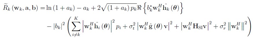
Objective function:
Main code:
% Inputs variables
K = 5; % Number of UEs
N = 8; % Number of RIS elements
Mt_trans = 5;
Mr_rec = 5;
rho = 0.33; % Amplifier efficiency of DRC-BS
samples = 2; % Number of channel realization
nbrOfSetups = 1; % Number of setups
N_iter = 10; % Number of iterations for optimization
tol = 1e-3; % Tolerence for comparasion
% Generating Parameter
B = 1e7 ; % Communication Bandwidth ( 10 MHz)
P_max = -30; % P_max_UE =[0,5,10,15,20,25,30](in dBm)
P_BS = 10 ^((9-30)/10); % Static circuit power consumption of DFRC-BS(9 dBm)
P_UE = 10 ^((9-30)/10); % Static power consumption of all UEs (9 dBm)
P_RIS = 1*(10 ^((0-30)/10)); % Static power consumption of an RIS(0 dBm)
C0_db = -30; % Path loss at reference distance d0 = 1 [m] (in db)
sigma_sqrdBm = -90; % Noise power at the DRC-BS (sigma_sqrdBm = -90 dBm)
sigma_sqr = 10 ^((sigma_sqrdBm-30)/10);
sigmaSI_sqrdBm = -110; % Self intereference (SI) attenuation level
sigmaSI_sqr = 10 ^((sigmaSI_sqrdBm-30)/10);
sigma_sqr_t=1; % Target radar cross section (RCS)
Gamma_tdB=5;Gamma_t=10^(Gamma_tdB/10); % Predefined target detection level (5 dB)
antennaSpacing=0.5; % half wavelength lambda/2
alpha_BS_Target = 2.2; % Path loss exponent for BS-target
alpha_RIS_Target = 2.2; % Path loss exponent for RIS-Target
alpha_BS_RIS = 2.7; % Path loss exponent for BS-target
Rician = 10 ^ (3/10); % Small scale fading for BS-RIS(Rician fading = 3dB)
alpha_UE_RIS = 2.4; % Path loss exponent for BS-target
alpha_UE_BS = 3.6; % Path loss exponent for BS-target
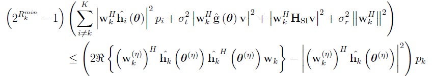
% QoS constraint on the individual rate
R_min = 0.5; % Minimum rate constraint for each UE
% RIS phase shift matrix
% start with random IRS beamforming matrix (Is feasible ?)
theta = 0 + 2*pi*rand(N,1); % Generate random phase
Phi = diag (exp(1i*theta)); % Generate diagional matrix
phi = diag (Phi); % Modify it to Row matrix
%% Main program starts
P=10 ^((P_max-30)/10); P1=[P,P,P,P,P];
EE_large=zeros(1,length(nbrOfSetups));
EE_large_unopt=zeros(1,length(nbrOfSetups));
% Loop over number of Setups
for Setups = 1: nbrOfSetups
% Setting up the scenario
[Loc_BS,Loc_Target,Loc_RIS,Loc_UE] = Scenario_setup(K);
EE_small=zeros(1,length(samples));
EE_small_unopt=zeros(1,length(samples));
% Inner loop for N_sim random simulations
for sim=1:samples
[g_t,g_r,d_t,d_r,G_t,G_r,h_r,h_d,w_0,h_s_i,h_theta,g_theta,w_k,v] = Channel_generator(C0_db,K,Mt_trans,Mr_rec,N,sigmaSI_sqr,antennaSpacing,alpha_BS_Target,alpha_RIS_Target,alpha_BS_RIS,alpha_UE_RIS,alpha_UE_BS,Rician,phi,Loc_BS,Loc_Target,Loc_RIS,Loc_UE);
%**************************************************************************
% Optimize receive beamforming for users
%**************************************************************************
% Objective function related to power optimization
J = zeros(1,N_iter);
% Random receive beamforming for users
w_k_initial=w_k;
[main_obj] = objective_main(K,w_k_initial,h_theta,P1,g_theta,h_s_i,v,sigma_sqr_t,sigma_sqr,rho,P_BS,P_UE,P_RIS);
EE_small_unopt(:,sim)=main_obj; % Store unoptimized EE for each small scale setup
for iter = 1 : N_iter
p = iter;
% Update a_k (eq.10) and z_k (eq.12)
[SINR,SINR_sqr,~,sum_rate] = Data_rate(K,w_k_initial,h_theta,P1,g_theta,h_s_i,v,sigma_sqr_t,sigma_sqr);
a=SINR; % SINR corresponding to optimized w_k
b=sqrt(1+a).*SINR_sqr;
% Solving problem (P4)
cvx_begin %quiet
variable w_k_opt(Mr_rec,K) complex
%variable Tx_beamforming(Mt_trans) complex
% Compute objective function (eq.11)
[obj_Rxbeam,~] = objective_Rxbeam(K,w_k_opt,h_theta,P1,g_theta,h_s_i,v,sigma_sqr_t,sigma_sqr,a,b);
obj = obj_Rxbeam;
maximize real(obj)
% constraints
% Individual Rate constraint (QoS) (eq.15)
for k=1:K
n = pow_pos((norm(w_k_opt(:,k)'*h_theta(:,k))),2)*P1(k);
i=zeros(1,1);
for mm=1:K
if mm~=k
i = i + pow_pos(norm(w_k_opt(:,k)'*h_theta(:,mm)),2)*P1(mm);
%b1(:,k) = b;
end
end
c1 = pow_pos(norm(w_k_opt(:,k)'*g_theta*v),2);
d1 = pow_pos(norm(w_k_opt(:,k)'*h_s_i*v),2);
e1 = pow_pos(norm(w_k_opt(:,k)'),2);
(2^(R_min)-1)*( i + c1*sigma_sqr_t + d1 + e1*sigma_sqr)...
<= ( 2*real ( w_k_initial(:,k)'*h_theta(:,k)*h_theta(:,k)'*w_k_opt(:,k))...
- pow_pos(norm(w_k_initial(:,k)'*h_theta(:,k)),2) )*P1(k);
end
% pow_pos(norm(...),2)
cvx_end
% cvx_status
if strcmp(cvx_status,'Solved') %|| strcmp(cvx_status,'Failed') || strcmp(cvx_status, 'Inaccurate/Solved')
w_k_initial = w_k_opt;
else
%w_k_opt = w_k_initial; % default value
end
w_k_initial;
w_k_opt;
% compute objective function
[obj_Rxbeam,obj_Rxbeam_converge] = objective_Rxbeam(K,w_k_initial,h_theta,P1,g_theta,h_s_i,v,sigma_sqr_t,sigma_sqr,a,b);
J(p) = real(obj_Rxbeam_converge);
% test stopping criterion
if N_iter > 1
abs(J(N_iter) - J(N_iter-1)) <= tol;
break;
end
end
[main_obj] = objective_main(K,w_k_opt,h_theta,P1,g_theta,h_s_i,v,Gamma_t,sigma_sqr,rho,P_BS,P_UE,P_RIS);
% Calculating the main objective corresponding to optimal power allocation
EE_small(:,sim)=main_obj; % Store EE for each small scale setup
end % End of channel samples loop
% Average EE
EE_small=mean(EE_small);
EE_small_unopt=mean(EE_small_unopt);
% Store EE for each large scale setup
EE_large(:,Setups)=EE_small*B;
EE_large_unopt(:,Setups)=EE_small_unopt*B;
end % End of nbrOfSetups loopS
% Average EE for all large scale setup
EE_RxBeam=mean(EE_large);
EE_RxBeam_unopt=mean(EE_large_unopt);
disp(EE_RxBeam/1e6);
disp(EE_RxBeam_unopt/1e6);
functions:
(1)
% Generation of overall channel
%function [Loc_BS,Loc_Target,Loc_RIS,Loc_UE] =Scenario_setup(K)
function [g_t,g_r,d_t,d_r,G_t,G_r,h_r,h_d,w_0,h_s_i,h_theta,g_theta,w_k,v] = Channel_generator(C0_db,K,Mt_trans,...
    Mr_rec,N,sigmaSI_sqr,antennaSpacing,alpha_BS_Target,alpha_RIS_Target,...
    alpha_BS_RIS,alpha_UE_RIS,alpha_UE_BS,Rician,phi,Loc_BS,Loc_Target,Loc_RIS,Loc_UE)

% Generate channel between BS-Target, RIS-target, BS-UE, UE-RIS & BS-RIS

        % Channel between BS and target: BS to target and target to BS

        d_BS_Target = norm (Loc_BS - Loc_Target); % BS-target link distance
        % Large scale fading (distance dependent path loss model)
        PL_BS_Target = C0_db -10 * alpha_BS_Target * log10 (d_BS_Target);
        pos_BS = Loc_BS(1) + 1i*Loc_BS(2);
        pos_Target = Loc_Target(1) + 1i*Loc_Target(2);

        % Angle from BS to target
        angleBS_Target = angle(pos_BS - pos_Target);
        g_t_LoS = (exp(1i*2*pi.*(0:Mt_trans-1)*sin(angleBS_Target)*antennaSpacing));
        % Composite channel
        g_t = sqrt(db2pow(PL_BS_Target)).*g_t_LoS;

        % Angle from target to BS
        angleTarget_BS = angle(pos_Target - pos_BS);
        g_r_LoS = (exp(1i*2*pi.*(0:Mr_rec-1)*sin(angleTarget_BS)*antennaSpacing));
        % Composite channel
        g_r = sqrt(db2pow(PL_BS_Target)).*g_r_LoS.';

       % Channel between RIS and target: RIS to Target and Target to RIS

        d_RIS_Target = norm (Loc_RIS - Loc_Target); % BS-target link distance
        % Large scale fading (distance dependent path loss model)
        PL_RIS_Target = C0_db -10 * alpha_RIS_Target * log10 (d_RIS_Target); % path loss
        pos_RIS = Loc_RIS(1) + 1i*Loc_RIS(2);
        pos_Target = Loc_Target(1) + 1i*Loc_Target(2);

        % Angle from RIS to Target
        angleRIS_Target = angle(pos_RIS - pos_Target);
        d_t_LoS = (exp(1i*2*pi.*(0:N-1)*sin(angleRIS_Target)*antennaSpacing));
        % Composite channel
        d_t = sqrt(db2pow(PL_RIS_Target)).*d_t_LoS;

        % Angle from Target to RIS
        angleTarget_RIS = angle(pos_Target - pos_RIS);
        d_r_LoS = (exp(1i*2*pi.*(0:N-1)*sin(angleTarget_RIS)*antennaSpacing));
        % Composite channel
        d_r = sqrt(db2pow(PL_RIS_Target)).*d_r_LoS.';

        % Channel between BS and RIS: BS to RIS and RIS to BS

        d_BS_RIS = norm (Loc_BS - Loc_RIS); % BS-target link distance
        % Large scale fading (distance dependent path loss model)
        PL_BS_RIS = C0_db -10 * alpha_BS_RIS * log10 (d_BS_RIS); % path loss
        pos_BS = Loc_BS(1) + 1i*Loc_BS(2);
        pos_RIS = Loc_RIS(1) + 1i*Loc_RIS(2);

        % Angle from BS to RIS
        angleBS_RIS = angle(pos_BS - pos_RIS);
        G_t_LoS = (exp(1i*2*pi.*(0:Mt_trans-1)*sin(angleBS_RIS)*antennaSpacing));
        G_t = sqrt(Rician/Rician+1)*(G_t_LoS.') + sqrt(1/Rician+1)*...
            (1/sqrt(2))*(randn(Mt_trans,N) + 1i*randn(Mt_trans,N));
        % Composite channel
        G_t = sqrt(db2pow(PL_BS_RIS)).*G_t.';

        % Angle from RIS to BS
        angleRIS_BS = angle(pos_RIS - pos_BS);
        G_r_LoS = (exp(1i*2*pi.*(0:Mr_rec-1)*sin(angleRIS_BS)*antennaSpacing));
        G_r = sqrt(Rician/Rician+1)*(G_r_LoS.') + sqrt(1/Rician+1)*...
            (1/sqrt(2))*(randn(Mr_rec,N) + 1i*randn(Mr_rec,N));
        % Composite channel
        G_r = sqrt(db2pow(PL_BS_RIS)).*G_r;

        % Channel from UL User Equipment (UE) to RIS

        % IRS-UE link distance
        d_UE_RIS = zeros(1,K); % BS-UE link distance
        %h_r=zeros(N,K);
        for kk=1:K

          d_UE_RIS(kk) = norm (Loc_UE(:,:,kk) - Loc_RIS);
          % Large scale fading (distance dependent path loss model
          PL_UE_RIS (kk) = C0_db -10 * alpha_UE_RIS * log10 (d_UE_RIS(kk)); % path loss
          % Small scale fading (Rayleigh fading)
          %h_r1(:,kk) = (1/sqrt(2))*(randn(N,1) + 1i*randn(N,1));
          % Composite channnel
          h_r(:,kk) = sqrt(db2pow(PL_UE_RIS(kk))).*(1/sqrt(2))*(randn(N,1) + 1i*randn(N,1));

        end

        % Channel from UL User Equipment (UE) to RIS

        d_UE_BS = zeros(1,K); % BS-UE link distance
       % h_d=zeros(Mr_rec,K);
        for  kk=1:K

            d_UE_BS(kk) = norm (Loc_UE(:,:,kk) - Loc_BS);
            % Large scale fading (distance dependent path loss model)
            PL_UE_BS(kk) = C0_db -10 * alpha_UE_BS * log10 (d_UE_BS(kk));
            % Small scale fading (Rayleigh fading)
            h_d1(:,kk) = (1/sqrt(2))*(randn(Mr_rec,1) + 1i*randn(Mr_rec,1));
            % Composite channnel
            h_d(:,kk) = sqrt(db2pow(PL_UE_BS(kk))).*h_d1(:,kk);

        end

        w_0=randn(Mr_rec,1) + 1i * randn(Mr_rec,1);
        h_s_i = sqrt(sigmaSI_sqr)*(randn(Mr_rec,Mt_trans) + 1i * randn(Mr_rec,Mt_trans));

        % Re-arranging the channel gains
            for k=1:K
                h_theta(:,k) = h_d(:,k) + G_r*diag(h_r(:,k))*phi;
                w_k(:,k)=randn(Mr_rec,1) + 1i * randn(Mr_rec,1); % Without MRC
                %w_k(:,k)=G_r*diag(h_r(:,k))*phi/norm(G_r*diag(h_r(:,k))*phi);% MRC with indirect (RIS path) receiving channel
            end
            %w_k=h_theta/norm(h_theta); % MRC with combined receiving channel
            g_r_theta = g_r + G_r*diag(d_r)*phi;
            g_t_theta = g_t + phi.'*diag(d_t)*G_t;
            g_theta = g_r_theta*g_t_theta; v = g_t'/norm(g_t);

end
(2)
% Function to generate transmit rate of each user

function [SINR,SINR_sqr,transmit_rate_UE,sum_rate] = Data_rate(K,w_k,h_theta,P_rand,g_theta,h_s_i,v,sigma_sqr_t,sigma_sqr)

% Calculating terms related to SINR expression
            for k=1:K
                a(k) = (norm(w_k(:,k)'*h_theta(:,k))^2)*P_rand(k);
                b=zeros(K,1);
                for mm=1:K
                    if mm~=k
                        b(mm,:) =  (norm(w_k(:,k)'*h_theta(:,mm))^2)*P_rand(mm);
                        b1(:,k) = b;
                    end
                end
                b1(:,k) = b;
                c(k) = norm(w_k(:,k)'*g_theta*v)^2;
                d(k) = (norm(w_k(:,k)'*h_s_i*v)^2);
                e(k)= norm(w_k(:,k)')^2 ;
                SINR(k) = (a(k))./(sum(b)+c(k)*sigma_sqr_t+d(k)+e(k)*sigma_sqr); % SINR
                SINR_sqr(k) = ( sqrt(a(k)) )./(sum(b)+c(k)*sigma_sqr_t+d(k)+e(k)*sigma_sqr); % SINR_sqr
                transmit_rate_UE(k)=log2(1+SINR(k));
            end
            sum_rate=sum(transmit_rate_UE);

end
(3)
% Function to generate an obj. function for receive beamformimg for users

function [obj_Rxbeam,obj_Rxbeam_converge] = obj_Rxbeam(K,w_k,h_theta,P_rand,g_theta,h_s_i,v,sigma_sqr_t,sigma_sqr,a,b)

% Calculating terms related to SINR (Auxiliary variable 'a') expression
for k=1:K
    n(k) = (square_pos(norm(w_k(:,k)'*h_theta(:,k))))*P_rand(k);
    i=zeros(1,1);
    for mm=1:K
        if mm~=k
            i = i + (square_pos(norm(w_k(:,k)'*h_theta(:,mm))))*P_rand(mm);
            %i1(:,k) = i;
        end
    end
    %i1(:,k) = i;
    c(k) = square_pos(norm(w_k(:,k)'*g_theta*v));
    d(k) = square_pos(norm(w_k(:,k)'*h_s_i*v));
    e(k)= square_pos(norm(w_k(:,k)')) ;
    obj_Rxbeam_converge1(k)=  log10 (1+a(k))-a(k) + 2*sqrt( (1+a(k)).*P_rand(k))...
        .*real( b(k).* (w_k(:,k)'*h_theta(:,k)) ) - (abs(b(k))^2)...
        .*(i + c(k)*sigma_sqr_t + d(k) + e(k)*sigma_sqr );
    obj_Rxbeam1(k)= 2*sqrt( (1+a(k)).*P_rand(k)).*real( b(k).* (w_k(:,k)'*h_theta(:,k)) )...
        - (abs(b(k))^2).*(i + c(k)*sigma_sqr_t + d(k) + e(k)*sigma_sqr );

end
obj_Rxbeam=sum(obj_Rxbeam1); %objective for optimization
obj_Rxbeam_converge=sum(obj_Rxbeam_converge1); % Objective for convergence


end
(4)
% Main objective function

function [main_obj] = objective_main(K,w_k,h_theta,P_rand,g_theta,h_s_i,v,sigma_sqr_t,sigma_sqr,rho,P_BS,P_UE,P_RIS)

% Calculating terms related to SINR expression
for k=1:K
    a(k) = (norm(w_k(:,k)'*h_theta(:,k))^2)*P_rand(k);
    b=zeros(K,1);
    for mm=1:K
        if mm~=k
            b(mm,:) =  (norm(w_k(:,k)'*h_theta(:,mm))^2)*P_rand(mm);
            b1(:,k) = b;
        end
    end
    b1(:,k) = b;
    c(k) = norm(w_k(:,k)'*g_theta*v)^2;
    d(k) = (norm(w_k(:,k)'*h_s_i*v)^2);
    e(k)= norm(w_k(:,k)')^2 ;
    SINR(k) = (a(k))./(sum(b)+c(k)*sigma_sqr_t + d(k)+e(k)*sigma_sqr); % SINR
    transmit_rate_UE(k)=log2(1+SINR(k));
end
sum_rate=sum(transmit_rate_UE);
main_obj=sum_rate/( sum(P_rand)+( (1/rho)*norm(v)^2 ) + P_BS + P_UE + P_RIS);

end
(5)
% Function to generate network topology

function [Loc_BS,Loc_Target,Loc_RIS,Loc_UE] =Scenario_setup(K)

Loc_BS = [5,0]; Loc_Target = [5,50];Loc_RIS = [10,10];

% randomly genertae K users in a cricle of radius 10 mt around [30,10]
         for kk=1:K
           r=rand*10;
           theta=rand*2*pi;
           x=r*cos(theta);
           y=r*sin(theta);
           Loc_UE(:,:,kk)= [30 + x, 10 + y];
         end
end
Output:
num. of constraints = 355
dim. of sdp var = 160, num. of sdp blk = 80
dim. of socp var = 320, num. of socp blk = 80
dim. of linear var = 165
SDPT3: Infeasible path-following algorithms
Status: Failed
Optimal value (cvx_optval): NaN
num. of constraints = 355
dim. of sdp var = 160, num. of sdp blk = 80
dim. of socp var = 320, num. of socp blk = 80
dim. of linear var = 165
SDPT3: Infeasible path-following algorithms
Status: Failed
Optimal value (cvx_optval): NaN
0.6233

0.1051
The failure in this case means that it could not solve the problem, due to encountering numerical difficulties. It does not necessarily mean that the problem is infeasible (or unbounded).
Try using Mosek, which is more numeri8cally robust than SDPT3 or SeDuMi. . Perhaps it will succeed In any event, pay attention to any Mosek warning messages about very large or near zero elements, which would be indicative of bad numerical scaling. If so, you should change the units in the problem so that all non-zero input data is within s small number of orders of magnitude of 1.
Can’t we solve using cvx then?
Now, I have to learn Mosek solver related coding skills. It may take time sir. And sometimes, same MATLAB version and same cvx version with diifferent computers solution is not getting means that only one system, my code is being solved and remaining systems it is showing solution is failed.
The statement
cvx_solver mosek
either before or within a CVX program specifies Mosek to be called as solver by CVX.
You can also use cvx_save_prefs if you have cvx_solver mosek prior to the CVX program. Then CVX will remember it for future MATLAB sessions.
cvx_solver mosek
% Solving problem (P4)
cvx_begin %quiet
                variable w_k_opt(Mr_rec,K) complex
                %variable Tx_beamforming(Mt_trans) complex
                 But getting error as:
Error using cvx_solver
Unknown, unusable, or missing solver: mosek
Error in Opt_beam_singlePower (line 93)
cvx_solver mosek
And I have added path to mosek solver in the command window
You have to rerun cvx_setup after adding mosek to your path. Make sure mosekdiag is successful before doing so.
And DON’T use quiet.
addpath F:\mosek\10.1\toolbox\R2017aom
mosekdiag
Matlab version : 9.12.0.2170939 (R2022a) Update 6
Architecture : PCWIN64
mosekopt path : F:\mosek\10.1\toolbox\R2017aom\mosekopt.mexw64
Error: could not load mosekopt.
Very likely the folder with shared libraries is not in the environment
variable PATH or you missed some operating-system-specific installation step.
Below is a more detailed debug info to help you identify the problem.
See the interface manual:
4 Installation — MOSEK Optimization Toolbox for MATLAB 10.1.28
for typical troubleshooting tips.
Detailed debug info:
Invalid MEX-file
‘F:\mosek\10.1\toolbox\R2017aom\mosekopt.mexw64’:
The specified module could not be found.
Error in mosekdiag (line 52)
[r, res] = mosekopt(‘version echo(0) nokeepenv’);
I am getting this error eventhough file is available
It means, as the message suggests, you didn’t add the folder with Mosek binaries to PATH, so it can’t find the Mosek DLLs.
See troubleshooting, second paragraph:
https://docs.mosek.com/latest/toolbox/install-interface.html#troubleshooting
Yes, I have installed mosek solver and previously it is being installed manually. Now, I have installed mosek solver and got license from the website , which is placed in C:\Users\ECE PHD\mosek.
Now, the mosekdiag is being verified and following has been displayed in the command window:
mosekdiag
Matlab version : 9.12.0.2170939 (R2022a) Update 6
Architecture : PCWIN64
mosekopt path : F:\mosek\10.1\toolbox\R2017aom\mosekopt.mexw64
MOSEK version : 10.1.22
Test linear solve: Success
Mosekopt works OK. You can use MOSEK in MATLAB.
Output:
Interior-point solution summary
Problem status : PRIMAL_AND_DUAL_FEASIBLE
Solution status : OPTIMAL
Primal. obj: -1.7629006462e+00 nrm: 3e+07 Viol. con: 6e-14 var: 0e+00 cones: 0e+00
Dual. obj: -1.7629006111e+00 nrm: 2e+04 Viol. con: 0e+00 var: 8e-09 cones: 3e-14
Optimizer summary
Optimizer - time: 0.03
Interior-point - iterations : 68 time: 0.03
Basis identification - time: 0.00
Primal - iterations : 0 time: 0.00
Dual - iterations : 0 time: 0.00
Clean primal - iterations : 0 time: 0.00
Clean dual - iterations : 0 time: 0.00
Simplex - time: 0.00
Primal simplex - iterations : 0 time: 0.00
Dual simplex - iterations : 0 time: 0.00
Mixed integer - relaxations: 0 time: 0.00
Status: Solved
Optimal value (cvx_optval): +1.7629
Here, the problem is solved , but optimal is giving NaN. I do not know the reason
NaN
0.0044
Please help in this regard
Please show all the CVX and solver output. And show us the exact command and output which resulted in NaN.