Why sometimes if I add constraints in the CVX problems, the optimal solution will be NaN and it can’t be continued?
It is possible that an original problem is feasible and when certain constraints. are added it becomes infeasible. Here is an example. Your problem may be more complicated, but the same phenomenon can occur.
cvx_begin
variable x
minimize(x)
x >= 0
cvx_end

Homogeneous problem detected; solution determined analytically.
Status: Solved
Optimal value (cvx_optval): +0
cvx_begin
variable x
minimize(x)
x >= 1
x <= 0
cvx_end
Calling SDPT3 4.0: 2 variables, 1 equality constraints
num. of constraints = 1
dim. of linear var = 2
SDPT3: Infeasible path-following algorithms
version predcorr gam expon scale_data
NT 1 0.000 1 0
it pstep dstep pinfeas dinfeas gap prim-obj dual-obj cputime0|0.000|0.000|1.1e+01|6.7e+00|2.0e+02| 1.000000e+01 0.000000e+00| 0:0:00| chol 1 1
1|0.930|1.000|7.4e-01|7.1e-02|5.3e+00| 2.829849e-01 1.045888e+01| 0:0:00| chol 1 1
2|0.287|1.000|5.3e-01|7.1e-03|5.5e+00| 2.054123e-02 1.093239e+02| 0:0:00| chol 1 1
3|0.040|1.000|5.0e-01|7.1e-04|4.1e+02| 1.972789e-03 4.836690e+04| 0:0:00| chol 1 1
4|0.007|1.000|5.0e-01|7.1e-05|5.9e+05| 2.134887e-04 6.959543e+08| 0:0:00| chol 1 1
5|0.001|1.000|5.0e-01|0.0e+00|8.2e+10| 2.155138e-05 9.591672e+14| 0:0:00| chol 1 1
6|0.000|1.000|5.0e-01|5.0e-01|1.1e+18| 2.157164e-06 1.315011e+23| 0:0:00|
sqlp stop: primal problem is suspected of being infeasiblenumber of iterations = 6
residual of primal infeasibility
certificate (y,Z) = 0.00e+00
reldist to infeas. <= 0.00e+00
Total CPU time (secs) = 0.04
CPU time per iteration = 0.01
termination code = 1
DIMACS: 5.0e-01 0.0e+00 5.0e-01 0.0e+00 -1.0e+00 8.5e-06
Status: Infeasible
Optimal value (cvx_optval): +Infx
x =
NaN
Thanks for your answer. The example you showed is an infesible problem, but I think the problem should be feasible after the constraints for variable u3_p are added, that’s why or I have something wrong with it?
Please copy and paste your program into your post, and use the preformmatted text.
I’m not sure what you are doing, but it looks like your (commented out) additional constraints for u3_p are constraining its elements to have magnitude <= 80. Why do you believe that is feasible? Have you produced a feasible solution for which the magnitude of elements of u3_p are <= 80? You haven’t provided a reproducible problem to allow us to more specifically assess your problem.
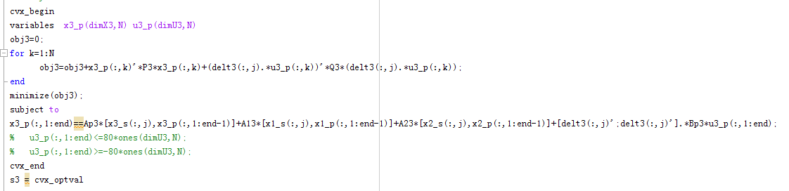
I paste the code following. I need to find the optimal solution in the constraint area to solve a constrained MPC. But it can’t.
Ts = 1;
A1 = 5*[-1/75 0.2;0.3 -1/75];
B1=5*[.878/75 .864/75;1.082/75 1.096/75];
C1=eye(2);D1=zeros(2);
Plant1 = ss(A1,B1,C1,D1);
[Ap1,Bp1,Cp1,Dp1] = ssdata(c2d(Plant1,Ts));
A2 = 5*[-1/75 0.1;0.2 -1/75];
B2 = 5*[.8781.8/75,.864.2/75;1.0821.8/75,1.096.2/75];
C2 = [1,0.5;-0.5,1];D2 = zeros(2);
Plant2 = ss(A2,B2,C2,D2);
[Ap2,Bp2,Cp2,Dp2] = ssdata(c2d(Plant2,Ts));
A3 = 6*[-1/75 0.3;0.1 -1/75];
B3 = 5*[.91.8/75,.864.2/75;1.11.8/75,1.1.2/75];
C3 = [0.8,-0.5;1,1];D3=zeros(2);
Plant3 = ss(A3,B3,C3,D3);
[Ap3,Bp3,Cp3,Dp3] = ssdata(c2d(Plant3,Ts));
A12 = [0.5,-0.2;0.3,0.5];
A13 = [0.3,0.2;0.5,-0.3];
A23 = [0.2,0.5;0.5,-0.2];
dimX1=size(A1,1);
dimU1=size(B1,2);
dimY1=size(C1,1);
dimX2=size(A2,1);
dimU2=size(B2,2);
dimY2=size(C2,1);
dimX3=size(A3,1);
dimU3=size(B3,2);
dimY3=size(C3,1);
N=5; M=3; %prediction and control horizon
simTime=100; %simulation time
x10=[1;5]; % initial states
x20=[3;-0.5];
x30=[-2;-3];
P1=ones(1,dimX1);
P1=5diag(P1);
P2=ones(1,dimX2);
P2=5diag(P2);
P3=ones(1,dimX3);
P3=5*diag(P3);
Q1=ones(1,dimU1);
Q1=diag(Q1);
Q2=ones(1,dimU2);
Q2=diag(Q2);
Q3=ones(1,dimU3);
Q3=diag(Q3);
P12 = ones(1,dimX2);
P12 = diag(P12);
P13 = ones(1,dimX3);
P130= diag(P13);
P23 = ones(1,dimX3);
P23 = diag(P23);
J=[];
s1=[]; s2=[]; s3=[];
x1 = zeros(dimX1,simTime+1);
x2 = zeros(dimX2,simTime+1);
x3 = zeros(dimX3,simTime+1);
x1_s=zeros(dimX1,simTime+1);
x1(:,1)=x10(:,1);
x1_s(:,1)=x10(:,1);
x2_s=zeros(dimX2,simTime+1);
x2(:,1)=x20(:,1);
x2_s(:,1)=x20(:,1);
x3_s=zeros(dimX3,simTime+1);
x3(:,1)=x30(:,1);
x3_s(:,1)=x30(:,1);
u1_e = zeros(dimU1,N);
u2_e = zeros(dimU2,N);
u3_e = zeros(dimU3,N);
x1_o = zeros(dimX1,simTime+1);
x2_o = zeros(dimX2,simTime+1);
x3_o = zeros(dimX3,simTime+1);
x1_o(:,1)=x10(:,1);
x2_o(:,1)=x20(:,1);
x3_o(:,1)=x30(:,1);
for j=1:simTime
disp(j)
% subsystem 1
cvx_begin
variables x1_p(dimX1,N) u1_p(dimU1,N)
obj1=0;
for k=1:N
obj1=obj1+x1_p(:,k)'P1x1_p(:,k)+u1_p(:,k)'Q1u1_p(:,k);
end
minimize(obj1);
subject to
x1_p(:,1:end)==Ap1*[x1_s(:,j),x1_p(:,1:end-1)]+Bp1*u1_p(:,1:end);
cvx_end
s1=cvx_optval
% subsystem 2
cvx_begin
variables x2_p(dimX2,N) u2_p(dimU2,N)
%minimize(Psum_square([x21;x22])+Qsum_square([u21;u22])+nu(N+2:2*(N),:)'u22);
obj2=0;
for k=1:N
obj2=obj2+x2_p(:,k)'P2x2_p(:,k)+u2_p(:,k)'Q2u2_p(:,k);
end
minimize(obj2);
subject to
x2_p(:,1:end)==Ap2[x2_s(:,j),x2_p(:,1:end-1)]+A12*[x1_s(:,j),x1_p(:,1:end-1)]+Bp2*u2_p(:,1:end);
cvx_end
s2 = cvx_optval
% subsystem 3
cvx_begin
variables x3_p(dimX3,N) u3_p(dimU3,N)
obj3=0;
for k=1:N
obj3=obj3+x3_p(:,k)'P3x3_p(:,k)+u3_p(:,k)'Q3u3_p(:,k);
end
minimize(obj3);
subject to
x3_p(:,1:end)==Ap3*[x3_s(:,j),x3_p(:,1:end-1)]+A13*[x1_s(:,j),x1_p(:,1:end-1)]+A23*[x2_s(:,j),x2_p(:,1:end-1)]+Bp3u3_p(:,1:end);
u3_p(:,1:end)<=80ones(dimU3,N);
u3_p(:,1:end)>=-80ones(dimU3,N);
cvx_end
s3 = cvx_optval
if j<13
u1_p(:,1)=u1_p(:,1);
u2_p(:,1)=u2_p(:,1);
u3_p(:,1)=u3_p(:,1);
elseif j<25&&j>13
u3_p(1,1)=-0.1;
elseif j<70&&j>60
u3_p(2,1)=1;
else
u1_p(:,1)=u1_p(:,1);
u2_p(:,1)=u2_p(:,1);
u3_p(:,1)=u3_p(:,1);
end
u1(:,j)=u1_p(:,1);
u2(:,j)=u2_p(:,1);
u3(:,j)=u3_p(:,1);
x1(:,j+1) = Ap1x1(:,j)+Bp1u1(:,j);
y1(:,j) = Cp1x1(:,j);
x2(:,j+1) = Ap2x2(:,j)+A12x1(:,j)+Bp2u2(:,j);
y2(:,j) = Cp2x2(:,j);
x3(:,j+1) = Ap3x3(:,j)+A13x1(:,j)+A23x2(:,j)+Bp3u3(:,j);
y3(:,j) = Cp3*x3(:,j);
x1_s(:,j+1) = x1(:,j+1);
x2_s(:,j+1) = x2(:,j+1);
x3_s(:,j+1) = x3(:,j+1);
u1_e = [u1_p(:,2:N),u1_p(:,N)];
x1_e = [x1_s(:,j),x1_p(:,2:N)];
u2_e = [u2_p(:,2:N),u2_p(:,N)];
x2_e = [x2_s(:,j),x2_p(:,2:N)];
u3_e = [u3_p(:,2:N),u3_p(:,N)];
x3_e = [x3_s(:,j),x3_p(:,2:N)];
% system estimation
x1_o(:,j+1) = Ap1x1_o(:,j)+Bp1u1(:,j);
x2_o(:,j+1) = Ap2x2_o(:,j)+A12x1_o(:,j)+Bp2u2(:,j);
x3_o(:,j+1) = Ap3x3_o(:,j)+A13x1_o(:,j)+A23x2_o(:,j)+Bp3*u3(:,j);
end
You have not provided all input data, for instance ss
Out of all of this, which CVX program reports infeasible which you claim is feasible? Why are you sure it is feasible?
That’s OK, ss is a function in control system. So maybe I have some misunderstanding about the cvx? I just want to find a optimal solution in my feasible area of the third CVX program, not a global optimal solution, can the CVX solve it?
I’m not an expert in MPC, but I can confidently say that not all MPC problems are feasible.
If CVX reports the problem is infeasible, that means that is has accepted the problem, and the solver determined it to be infeasible. If CVX claims to have solved the problem, it will be a globally optimal solution.
If you solve the problem without the +/- 80 bounds, is there a solution? Does that solution satisfy the +/- 80 bound constraints? I presume not. To see how close there is to being a solution satisfying those constraints, remove those constraints, and replace the objective with norm(u3_p(:),inf) . If cvx_optval > 80, your original problem with the bounds is infeasible.
By the way, I think those constraints can be stated more simply as-80 <= u3_p <= 80
Yes,you are right. There are solutions out of the constraints. But I need to find the solutions in the constraint area,so I can’t solve it with CVX?But if it can’t,the constraints may be no use in CVX?
Maybe I have found my problem,thank you very much for your answers.
If you “can’t” solve it (this) in CVX, you can’t solve it with anything. Unless the problem is borderline feasible, or is numerically very bad, either it is infeasible or it isn’t. The same model entered though a different modeling or solver input system would also find the problem to be infeasible if CVX did. If (in)feasibility is borderline, then different solver feasibility tolerance might result in a different conclusion. Similarly if the model is numerically very bad.