HELP! How to implement following function in CVX?

[Sarah]

Hello everyone! I am a new to cvx. Could some help me to implement following function in CVX?

Here is my code:
h_temp=zeros(2,2);
P0=1;
for i=1:carrierno1
r=[out1(i,trainingno+1:end);out2(i,trainingno+1:end)];
h_temp=[ha1(i) ha2(i);ha3(i) ha4(i)];
h_temp1=abs(sum(h_temp(:,1)))^2;
h_temp2=abs(sum(h_temp(:,2)))^2;
cvx_begin
variable p
maximize(SINR1+SINR2)
subject to
p1= sqrt(P0/(1+p));
p2= sqrt(P0p/(1+p));
SINR1=p1^2h_temp1/(p2^2h_temp2+2noise_variance^2);
SINR2=p2^2h_temp2/(2noise_variance^2);
cvx_end
There are so many errors, could you help me?

[Erling (Erling D.Andersen)]

Your model has a nonlinear equality so this is nonconvex model which is unsolvable as is with CVX since it only handles convex models.

[Mark_L_Stone]

Because p_1 and p_2 only appear as p_1^2 and p_2^2, p_1^2 and p_2^2 can be replaced by variables p1sq, p2sq declared as
variables p1sq p2sq
The constraints then become

p1sq + p2sq == 1
0 <= p1sq <= Pmax
0 <= p2sq <= Pmax

This formulation would be a Fractional Linear Programming problem, but for the (additive) non-fractional term involving p2sq in the objective function. Linear Fractional Programs can be formulated and solved in CVX via the transformation described in 4.3.2 “Linear-fractional programming” of http://stanford.edu/~boyd/cvxbook/bv_cvxbook.pdf I leave it to you whether the Linear Fractional Programming reformulationcan be adapted to tjhis problem.

If not, and If you are willing to try an iterative procedure which calls CVX repeatedly, and is essentially a local optimization algorithm, with limited guarantee of convergence, you can try How to handle nonlinear equality constraints? . To apply this procedure to your problem, you would write two inequality constraints
p_1^2 + p_2^2 \le 1

p_1^2 + p_2^2 \ge 1

The first of these can be directly entered into CVX. The second of these could be handled by the convex-concave procedure described in the link. Stephen Boys A more detailed paper co-authored by Stephen Boyd is Variations and extension of the convex–concave procedure . There are example of the convex concave procedure using CVX to solve the convex sub-problems at https://web.stanford.edu/~boyd/software/cvx_ccv_examples/ .

However, you may be better off using a non-convex solver. Given that your problem only has 2 variables, it might be easily solvable to provable global optimality by a branch and bound global optimizer, such as BARON or YALMIP’s BMIBNB, both of which can be called from MATLAB.

[Sarah]

Thank you very much!

[Sarah]

Thank you for your help!
I have tried the first method “Linear Fractional Programs”,but I still have something unknown.
There is the simplified formulation:

so the objective function will be fractional-quadratic problem, how to solve it?

[Mark_L_Stone]

I wrote “I leave it to you whether the Linear Fractional Programming reformulation can be adapted to this problem.” That is still the case. So you can either figure out whether that can be done, don’t use CVX (rather, use a non-convex solver) per @Erling (that might be the best option) , or try the convex concave procedure.

[Sarah]

Hello again!
I have rewrote the above function, and I am sure that it is a convex models.

so I rewrite the primary optimization problem (13) by the following quadratic transform with introduced
variables .

[Sarah]

Meets the preceding text

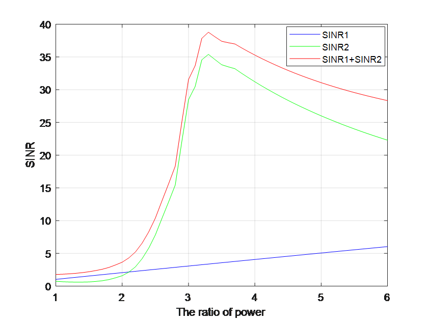
I solve the above reformulated convex optimization problem by CVX，and the status is ‘Solved’.But the optimal value is not exact. By following picture, the optimal p for primary problem is 3.2(it is a numerical modeling)

When I change the initialize p, the final value will change, too. But the optimal p is only for this problem. Why is it happening ?How can I find a feasible initialize p?
Here is the code and CVX display:
QAMbit1=4;
QAMbit2=16;
L=10000;
SNR=22;
SNR_V=10.^(SNR/10);
P0 =1;
N0=P0./SNR_V;
sigma = sqrt(N0/2);
n=sigmarandn(1,L)+sigma1i*randn(1,L);
%%
%initialization
p=3; %equal allocation
p2= P0./(1+p);
p1= p.*P0./(1+p);

rng(100)
decimal_data1=randi([0,QAMbit1-1],1,L);
data_bit1=de2bi(decimal_data1);
decimal_data2=randi([0,QAMbit2-1],1,L);
data_bit2=de2bi(decimal_data2);
const1=qammod([0:QAMbit1-1],QAMbit1);
power1=sum(abs(const1).^2)/QAMbit1;
qamdata1=qammod(decimal_data1,QAMbit1)/sqrt(power1);
const2=qammod([0:QAMbit2-1],QAMbit2);
power2=sum(abs(const2).^2)/QAMbit2;
qamdata2=qammod(decimal_data2,QAMbit2)/sqrt(power2);

H=[0.5063 0.5017;
0.5118 0.4907];
HH1=(H(1,1)+H(2,1))^2;
HH2=(H(1,2)+H(2,2))^2;
Y1=sqrt(p1)(H(1,1)+H(2,1))qamdata1;
Y2=sqrt(p2)(H(1,2)+H(2,2))qamdata2;
Y=Y1+Y2+n;
%SIC解码
r=Ysqrt(power1)/(sqrt(p1)(H(1,1)+H(2,1)));
recoverdata1=qamdemod(r,QAMbit1);
r1=qammod(recoverdata1,QAMbit1)/sqrt(power1);
r2=Y-sqrt(p1)(H(1,1)+H(2,1))r1;
rr2=r2sqrt(power2)/(sqrt(p2)(H(1,2)+H(2,2)));
recoverdata2=qamdemod(rr2,QAMbit2);
ep=mean(abs(recoverdata1-decimal_data1).^2);%imperfect SIC
%compute SINR
SINR1=p1HH1/(p2HH2+N0);
SINR2=p2HH2/(epp1HH1+N0);
SINR=SINR1+SINR2;
%put into formula
sita1=sqrt(p1HH1)/(p2HH2+N0);
sita2=sqrt(p2HH2)/(epp1HH1+N0);
cvx_begin
variables p1 p2
L=2sita1sqrt(p1HH1)-sita1^2(p2HH2+N0)+2sita2sqrt(p2HH2)-sita2^2*(epp1HH1+N0);
maximize(L)
subject to
p1 + p2 == 1
0 <= p1
0 <= p2 <=0.5
cvx_end
%%
p=p1/p2

Calling SDPT3 4.0: 11 variables, 5 equality constraints
For improved efficiency, SDPT3 is solving the dual problem.

num. of constraints = 5
dim. of sdp var = 4, num. of sdp blk = 2
dim. of linear var = 5

---

SDPT3: Infeasible path-following algorithms

---

version predcorr gam expon scale_data
HKM 1 0.000 1 0
it pstep dstep pinfeas dinfeas gap prim-obj dual-obj cputime

0|0.000|0.000|2.5e+00|1.0e+01|9.0e+02| 4.010693e+01 0.000000e+00| 0:0:00| chol 1 1
1|1.000|0.977|2.2e-07|3.4e-01|6.2e+01| 3.704702e+01 1.460156e+00| 0:0:01| chol 1 1
2|1.000|1.000|5.3e-07|1.0e-02|5.8e+00| 7.133830e+00 1.549022e+00| 0:0:01| chol 1 1
3|1.000|0.977|8.3e-08|1.2e-03|1.2e+00| 4.654259e+00 3.432345e+00| 0:0:01| chol 1 1
4|0.938|1.000|4.7e-08|1.0e-04|8.5e-02| 3.811250e+00 3.726764e+00| 0:0:01| chol 1 1
5|0.972|0.970|3.8e-09|1.3e-05|3.4e-03| 3.750478e+00 3.747223e+00| 0:0:01| chol 1 1
6|0.974|0.940|4.2e-09|1.7e-06|1.4e-04| 3.748246e+00 3.748120e+00| 0:0:01| chol 1 1
7|0.955|0.952|6.5e-10|8.3e-08|6.9e-06| 3.748183e+00 3.748177e+00| 0:0:01| chol 1 1
8|1.000|0.989|3.7e-10|1.0e-09|8.7e-07| 3.748180e+00 3.748180e+00| 0:0:01| chol 1 1
9|1.000|1.000|6.4e-12|7.4e-11|1.5e-08| 3.748180e+00 3.748180e+00| 0:0:01|
stop: max(relative gap, infeasibilities) < 1.49e-08

number of iterations = 9
primal objective value = 3.74817992e+00
dual objective value = 3.74817990e+00
gap := trace(XZ) = 1.54e-08
relative gap = 1.81e-09
actual relative gap = 1.74e-09
rel. primal infeas (scaled problem) = 6.40e-12
rel. dual " " " = 7.44e-11
rel. primal infeas (unscaled problem) = 0.00e+00
rel. dual " " " = 0.00e+00
norm(X), norm(y), norm(Z) = 4.9e+00, 1.0e+00, 2.3e+00
norm(A), norm(b), norm© = 4.6e+00, 4.6e+00, 2.7e+00
Total CPU time (secs) = 0.98
CPU time per iteration = 0.11
termination code = 0
DIMACS: 7.6e-12 0.0e+00 1.0e-10 0.0e+00 1.7e-09 1.8e-09

---

Status: Solved
Optimal value (cvx_optval): +1.96063

p =

3.4692

[Mark_L_Stone]

I don’t understand what you are doing, or why the solution calculated by the solver and reported by CVX as solved to opimality, is not close enough to what you believe to be the correct solution to satisfy you.

In what way is the solution not accurate enough? is the optimal objective value close enough? if so, perhaps the solution is wither not unique, or the objective is very flat in the region of the optimum, meaning that argument values which are not very close in distance from the optimal might be very close in objective value.

From a casual glance at your code, i see many random numbers are generated. Are you comparing what you consider to be the correct answer, using the same random numbers as used in the problem provided to CVX? If you re-run your entire program, different random numbers will be generated, and therefore a different problem instance provided to CVX, which presumably could have a different solution.